OpenCV 實作
OpenCV 影像讀取、顯示、色彩處理與電腦視覺實作筆記。
- Updated —
- June 23, 2026
- Topics —
- OpenCV, 電腦視覺
OpenCV 基礎套件
讀取檔案
import cv2
from matplotlib import pyplot as plt

img0 = cv2.imread('./image/SpongeBob.jpg', cv2.IMREAD_GRAYSCALE)  # same
# img0 = cv2.imread('./image/SpongeBob.jpg', 0)    # 0 灰階

img1 = cv2.imread('./image/SpongeBob.jpg', cv2.IMREAD_COLOR)    # 1 BGR,  1 可省略(原圖)
# img1 = cv2.imread('./image/SpongeBob.jpg', 1)                 # 1 BGR,  1 可省略(原圖)

cv2.imshow('SpongeBob Gray uint8', img0)  # cv2.imshow(視窗名稱, 圖片變數) 視窗名稱不能重複
# cv2.waitKey(0)
cv2.imshow('SpongBob Color uint8', img1)             # unit8
# cv2.imshow('SpongBob Color *256', img1*256)          # unit16
cv2.imshow('SpongBob Color 1/256 float', img1/256)   # floating 0.0 ~ 1.0

cv2.waitKey(0)                                       # 0 wait for anykey任意按鍵, try 3000 ms
cv2.destroyAllWindows()  #釋放記憶體
cv2.waitKey(1)  # 打給ios系統看的
讀取與顯示
#讀取
灰階
img0 = cv2.imread('./image/SpongeBob.jpg', cv2.IMREAD_GRAYSCALE)
img0 = cv2.imread('./image/SpongeBob.jpg', 0)

彩色
img1 = cv2.imread('./image/SpongeBob.jpg', cv2.IMREAD_COLOR)
img1 = cv2.imread('./image/SpongeBob.jpg', 1)

保留Alpha
img1 = cv2.imread('./image/SpongeBob.jpg', cv2.IMREAD_UNCHANGED)
img1 = cv2.imread('./image/SpongeBob.jpg', -1)

#顯示
# cv2.imshow(視窗名稱, 圖片變數)

cv2.imshow('SpongBob Color uint8', img1)
print(img1.dtype)

img1 的資料型態是 uint8 所以可以存0 ~255

除法
cv2.imshow('SpongBob Color 1/256 float', img1/256)

除以256之後 可以存0 ~ 0.996
OpenCV 對 float 圖片的規則:0=黑 1=白

乘法
cv2.imshow('SpongBob Color *256', img1*256)
因為uint8(NumPy資料型態) 所以大於255的數值會產生溢位 溢位會從0開始循環,所以結果數值會亂掉

NumPy:
超過範圍 → 繞回去 (Overflow)
OpenCV:
超過範圍 → 卡在最大值 (Saturation)

但如果是用unit16
img16 = img1.astype('uint16')
img16 = img16 * 256
0 ~ 65535cv2.waitKey(0)
永遠等待
直到按下鍵盤
cv2.waitKey(3000)
等待 3000 ms
= 3 秒
cv2.destroyAllWindows()
把所有 OpenCV 視窗關閉。
cv2.waitKey(1) #再多打一次給作業系統 表示真的要將視窗關閉資料型態-NumPy
| dtype | 數值範圍 |
| uint8 | 0\~255 |
| uint16 | 0\~65535 |
| float32/64 | 0.0\~1.0 |
| 名稱 | 描述 | 簡寫 |
| `np.bool_` | 用一個位元組儲存的布林值(True 或 False) | `'b'` |
| `np.int8` | 1 位元組整數,範圍:-128 \~ 127 | `'i1'` |
| `np.int16` | 2 位元組整數,範圍:-32768 \~ 32767 | `'i2'` |
| `np.int32` | 4 位元組整數,範圍:-2³¹ \~ 2³¹-1 | `'i4'` |
| `np.int64` | 8 位元組整數,範圍:-2⁶³ \~ 2⁶³-1 | `'i8'` |
| `np.uint8` | 1 位元組無符號整數,範圍:0 \~ 255 | `'u1'` |
| `np.uint16` | 2 位元組無符號整數,範圍:0 \~ 65535 | `'u2'` |
| `np.uint32` | 4 位元組無符號整數,範圍:0 \~ 2³²-1 | `'u4'` |
| `np.uint64` | 8 位元組無符號整數,範圍:0 \~ 2⁶⁴-1 | `'u8'` |
| `np.float16` | 半精度浮點數:16 位元(1 位符號、5 位指數、10 位尾數) | `'f2'` |
| `np.float32` | 單精度浮點數:32 位元(1 位符號、8 位指數、23 位尾數) | `'f4'` |
| `np.float64` | 雙精度浮點數:64 位元(1 位符號、11 位指數、52 位尾數) | `'f8'` |
| `np.complex64` | 複數,由兩個 `float32` 組成(實部 + 虛部) | `'c8'` |
| `np.complex128` | 複數,由兩個 `float64` 組成(實部 + 虛部) | `'c16'` |
| `np.object_` | Python 物件型別 | `'O'` |
| `np.string_` | 位元組字串(bytes) | `'S'` |
| `np.unicode_` | Unicode 字串 | `'U'` |
img0 = cv2.imread(‘./image/SpongeBob.jpg’, cv2.IMREAD_GRAYSCALE) # same
img0 = cv2.imread(‘./image/SpongeBob.jpg’, 0) # 0 灰階
img1 = cv2.imread(‘./image/SpongeBob.jpg’, cv2.IMREAD_COLOR) # 1 BGR, 1 可省略(原圖)
0 灰階
print(f’{“=”*15} {“gray”} {“=”*15}\nshape\t: {img0.shape}\n’ f’ndim\t: {img0.ndim}\n’ f’size\t: {img0.size}\n’ f’dtype\t: {img0.dtype}\n’ f’type\t: {type(img0)}\n’)
1 RGB
print(f’{“=”*15} {“color”} {“=”*14}\nshape\t: {img1.shape}\n’ f’ndim\t: {img1.ndim}\n’ f’size\t: {img1.size}\n’ f’dtype\t: {img1.dtype}\n’ f’type\t: {type(img1)}’)
print(img1[0,0]) 可以直接查看左上角的像素
圖片讀取近來都是NumPy的資料型態
=============== gray ===============<br>shape	: (560, 840)<br>ndim	: 2 (二維陣列)<br>size	        : 470400 (560\*840)<br>dtype	: uint8<br>type	: \<class 'numpy.ndarray'\>  numpy.array是一個矩陣
=============== color ==============<br>shape	: (560, 840, 3)  三個通道 BGR<br>ndim	: 3 (三維陣列)<br>size        	: 1411200 (560\*840\*3)<br>dtype	: uint8<br>type	: \<class 'numpy.ndarray'\> numpy.array是一個矩陣
\[ 37 145  56\]   → 左上角的像素

\[<br>\[123, 50, 200, ...\],<br>\[ 30,255, 100, ...\],<br>...<br>\]
每一個數值的範圍是0\~255

## BGR → RGB & 畫圖
```python
import numpy as np
import cv2
from matplotlib import pyplot as plt

讀取彩色圖檔
img_bgr = cv2.imread('./image/baby.jpg', 1)      # 使用 OpenCV 讀取圖檔

[B,G,R] -> [R,G,B]
img_rgb = cv2.cvtColor(img_bgr, cv2.COLOR_BGR2RGB)    # 將 BGR 圖片轉為 RGB 圖片
# img_rgb = img_bgr[:,:,::-1]                         # 或是這樣亦可

-----------畫圖------------
1. 建立畫布 寬16英吋 長9英吋
plt.figure(figsize=(16, 9))                # 使用 Matplotlib 顯示圖片

2.創建一個放圖的表格 subplot(121): 1列 2欄 第一張
plt.subplot(1,2,1), plt.imshow(img_rgb), plt.title('plt rgb')

plt.subplot(122), plt.imshow(img_bgr), plt.title('cv2 bgr in matplotlib')
plt.imshow

cv2.imshow('bgr', img_bgr)                     # cv2 show bgr
cv2.waitKey(0)                                 # 0 wait for anykey任意按鍵, try 3000
cv2.destroyAllWindows()
cv2.waitKey(1)
OpenCV 彩色通道的順序為 BGR
matplotlib 的順序為 RGB
所以在畫圖之前 一定要先將圖片 BGR 轉成RGB
subplot(121)
+———+———+
| 圖1 | 圖2 |
+———+———+
plt.imshow(img_rgb) 要顯示的圖片名稱
plt.title(‘plt rgb’) 視窗名稱
plt rgb
┌───────────────┐
│ │
│ 圖片 │
│ │
└───────────────┘
存檔壓縮
import cv2

#讀取灰階檔案
img0 = cv2.imread('./image/baby.jpg', 0)    # 0 灰階
cv2.imwrite('./image/baby01.jpg', img0)

# cv2.imwrite(檔案路徑, 圖片變數, [cv2.IMWRITE_JPEG_QUALITY, 品質值])
# 設定 JPEG 圖片品質為 90(可用值為 0 ~ 100)
cv2.imwrite('./image/baby02.jpg', img0, [cv2.IMWRITE_JPEG_QUALITY, 90])

# 設定 PNG 壓縮層級為 5(可用值為 0 ~ 9)
cv2.imwrite('./image/baby03.png', img0, [cv2.IMWRITE_PNG_COMPRESSION, 5])
JPEG 品質範圍 → 有損壓縮
| 品質 | 說明 |
| 100 | 幾乎不壓縮 |
| 95 | 常用 |
| 90 | 品質佳、檔案較小 |
| 80 | 網頁常用 |
| 50 | 明顯失真 |
| 0 | 品質最差 |
| 壓縮率 | 特性 |
| 0 | 不壓縮 |
| 1 | 很快 |
| 3 | 常用 |
| 5 | 平衡 |
| 9 | 最小檔案 |
檢查圖片有沒有讀取成功
import cv2
import sys

img = cv2.imread('./image/lenaColor.png')    #調用cv2.imread()讀取影像

if img is None:
sys.exit('無法讀取影像...') # 印出文字後 立刻停止程式
else :
    print(f'img shape : {img.shape}')
    cv2.imshow('Image Show', img)           #調用cv2.imshow() 顯示讀取進來的影像
cv2.waitKey(0)
cv2.destroyAllWindows()
cv2.waitKey(1)
單一像素
#指定pix位置 y, x
a=100
px = img[a, a]             # RGB 100, 100 的值 取得 (100,100) 位置的像素
print(px)                  #顯示BGR顏色數值

result: (120, 145, 200)

blue = img[a, a, 0]        # 0:Blue, 1:Green, 2:Red 指定 x, y座標上 0 通道到數值 第三欄是0所以指定的是藍色
print(blue)

result: (120)

img[a, a] = [0, 0, 0]      # 指定圖片像素值[B, G, R] 給 0 值 改三個通道改成黑色
print(img[a, a])

result: [0 0 0]
# 基於numpy的資料格式指定物件
img = cv2.imread('./image/lenaColor.png') #調用cv2.imread()讀取影像
print(f'(10, 10, 2)像素的紅色數值\t: {img[10, 10, 2]}\n') # 0:Blue, 1:Green, 2:Red
#修改像素值 itemset
img[10, 10, 2] = 120 # set (10, 10, 2) = 120
print(f'after img[10,10,2]\t\t: {img[10, 10, 2]} \n') # 120
print(f'img.shape\t\t\t: {img.shape}\n' # 行、列、通道;圖像長寬與通道數(channels),可以判斷灰階或彩圖
f'img.size\t\t\t: {img.size:,}\n' # 像素數量*通道數
f'img.dtype\t\t\t: {img.dtype}') # 像素資料型態 uint8(0~255)(10, 10, 2)像素的紅色數值 : 226
after img[10,10,2] : 120
img.shape : (512, 512, 3)
img.size : 786,432
img.dtype : uint8
補充 — 跳脫字元
| 字元 | 意義 |
| `\n` | 換行 (New Line) |
| `\t` | Tab |
| `\\` | 顯示反斜線 `\` |
| `\'` | 顯示單引號 `'` |
| `\"` | 顯示雙引號 `"` |
裁切圖片
#分割圖像區域
logo = img[100:400, 150:415]    # y1 :  y2, x1 : x2
print(f'logo size : {logo.shape}')

cv2.imshow('Image Show', logo)
cv2.waitKey(0)
cv2.destroyAllWindows()
cv2.waitKey(1)
import numpy as np
import cv2
img = cv2.imread('./image/assassin.jpg')
cropped = img[100:400, 200:500]
cv2.imshow('Original', img)
cv2.imshow('cropped', cropped)
print(f'cropped size : {cropped.shape}')
cv2.waitKey(0)
cv2.destroyAllWindows()
cv2.waitKey(1)先將三個通道拆開,在案ˋ想要的順序黏回去 拆通道 b, g, r = cv2.split(檔案變數) b = img[:,:,0]; g = img[:,:,1]; r = img[:,:,2] 黏通道 cv2.merge([r,g,b])
img = cv2.imread('./image/assassin.jpg')

b, g, r = cv2.split(img)     # 分割通道
# b = img[:,:,0];  g = img[:,:,1];  r = img[:,:,2]  #也可以陣列指定通道分割

print(f'{b.shape}\n\n'
      f'r =\n{r}')
result:
(489, 800)
r =
[[ 94  94  93 ... 153 154 154]
 [ 96  95  93 ... 152 153 153]
 [ 98  97  94 ... 152 152 153]
 ...
 [ 85  76  71 ...  97  76  60]
 [ 85  76  77 ... 107  83  56]
 [ 67  72  90 ...  80  71  55]]

cv2.imshow('b', b)  #灰階
cv2.imshow('g', g)  #灰階
cv2.imshow('r', r)  #灰階

cv2.imshow('rgb', cv2.merge([r,g,b]))   #把三個通道黏回去
cv2.imshow('bgr', cv2.merge([b,g,r]))

cv2.waitKey(0)
cv2.destroyAllWindows()
cv2.waitKey(1)
要顯示單一通道的顏色 要先取出單一通道 然後再讓其他兩個通道變成0黏回去
import numpy as np

b, g, r = cv2.split(img)

zero = np.zeros_like(b)

blue_img = cv2.merge((b, zero, zero))

cv2.imshow("Blue Color", blue_img)
基礎繪圖
直線
cv2.line**( 影像, 開始座標, 結束座標, 顏色, 線條寬度 )**
import cv2
import numpy as np

#建立一個512*512的彩色圖片,預設像素值=0 舊式建立一個黑色的畫布
gc = np.zeros((512, 512, 3), dtype='uint8')

#畫線 (影像, 起始座標, 結束座標, 顏色, 線條寬度)
cv2.line(gc, (10, 50), (400, 300), (255, 0, 0), 15)
cv2.line(gc, (100, 50), (400, 500), (0, 0, 255), 3)
cv2.imshow('draw', gc)

cv2.waitKey(0)
cv2.destroyAllWindows()
cv2.waitKey(1)
import cv2
import numpy as np
gc = np.zeros((512, 512, 3), dtype='uint8')
cv2.arrowedLine(gc, (10, 50), (400, 300), (255, 0, 0), 5, tipLength = 0.05)
cv2.arrowedLine(gc, (100, 50), (400, 500), (0, 0, 255), 3, tipLength = 0.2)
cv2.imshow('draw', gc)
cv2.waitKey(0)
cv2.destroyAllWindows()
cv2.waitKey(1)箭頭線
cv2.arrowedLine ( 影像, 開始座標, 結束座標, 顏色, 線條寬度[…..] )
import cv2
import numpy as np

#產生一個512*512的黑色畫布
gc = np.zeros((512, 512, 3), dtype='uint8')

# cv2.arrowedLine(影像, 起始座標, 結束座標, 顏色, 線寬(thickness), 箭頭長度比例tipLength =  )
cv2.arrowedLine(gc, (10, 50), (400, 300), (255, 0, 0), 5, tipLength = 0.05) # tipLength為線長的5%
cv2.arrowedLine(gc, (100, 50), (400, 500), (0, 0, 255), 3, tipLength = 0.2) # tipLength為線長的20%
cv2.imshow('draw', gc)

cv2.waitKey(0)
cv2.destroyAllWindows()
cv2.waitKey(1)
矩形
cv2.rectangle(影像, 頂點座標, 對向頂點座標, 顏色, 線條寬度)
gc = np.zeros((512, 512, 3), dtype='uint8')

# cv2.rectangle(影像, 左上角座標, 右下角座標, 顏色的, 線寬)  #線寬為負值:表示實心框 圖形填滿
cv2.rectangle(gc, (30, 50), (200, 280), (0, 0, 255), 5)
cv2.rectangle(gc, (100, 200), (296, 376), (234, 151, 102), -5)   # -1 : 實心框
cv2.imshow('draw', gc)

cv2.waitKey(0)
cv2.destroyAllWindows()
cv2.waitKey(1)
圓形
cv2.circle ( 影像, 圓心座標, 半徑, 顏色, 線條寬度 )
gc = np.zeros((512, 512, 3), dtype='uint8')

# cv2.circle(影像, 圓心座標, 半徑, 顏色, 線寬)
cv2.circle(gc, (200, 100), 80, (255, 255, 0), 2)
cv2.circle(gc, (280, 180), 60, (147, 147, 147), -3)
cv2.imshow('draw', gc)

cv2.waitKey(0)
cv2.destroyAllWindows()
cv2.waitKey(1)
橢圓
cv2.ellipse ( 影像, 中心座標, (長軸, 短軸), 旋轉角度, 起始角度, 結束角度, 顏色, 線條寬度 )
gc = np.zeros((512, 512, 3), dtype='uint8')

# ellipse(影像, 中心座標, (長軸, 短軸), 旋轉角度, 起始角度, 結束角度, 顏色, 線寬)
# 起始角度0度的位置在12點鐘方向,以逆時針方向旋轉
cv2.ellipse(gc, (200, 100), (80, 40), 45, 0, 360, (80, 127, 255), 5)
cv2.ellipse(gc, (250, 300), (90, 50), 0, 0, 270, (44, 141, 108), -1)
cv2.imshow('draw', gc)

cv2.waitKey(0)
cv2.destroyAllWindows()
cv2.waitKey(1)
多邊形折線
cv2.polylines ( 影像, 頂點座標, 封閉型, 顏色, 線條寬度 )
gc = np.zeros((512, 512, 3), dtype='uint8')

#設定頂點座標 4個點
pts = np.array(((100,50), (100,200), (170,300), (300,50)))

# cv2.polylines(影像, [頂點座標], 是否封閉, 顏色, 線寬)
# 0 : 不封閉   1 : 封閉
cv2.polylines(gc, [pts], 0, (105, 105, 255), 2)  #True:頭尾相連; False:頭尾不相連 #0改1,就變封閉圖形
cv2.imshow('draw', gc)

cv2.waitKey(0)
cv2.destroyAllWindows()
cv2.waitKey(1)
文字
cv2.putText(影像, 文字, 座標, 字型, 大小, 顏色, 線條寬度, 線條種類)
import numpy as np
import cv2

#建立 540 * 1180 的白色畫布
gc = np.full((540, 1180, 3), 255, dtype='uint8')  # 用(B, G, R) = (255, 255, 255): 白色填滿畫布
# gc = cv2.imread('./image/baby.jpg')    # 0 灰階

font = [cv2.FONT_HERSHEY_SIMPLEX,
        cv2.FONT_HERSHEY_PLAIN,
        cv2.FONT_HERSHEY_DUPLEX,
        cv2.FONT_HERSHEY_COMPLEX,
        cv2.FONT_HERSHEY_TRIPLEX,
        cv2.FONT_HERSHEY_COMPLEX_SMALL,
        cv2.FONT_HERSHEY_SCRIPT_SIMPLEX,
        cv2.FONT_HERSHEY_SCRIPT_COMPLEX ]

for idx, f in enumerate(font):  #for idx, f in enumerate(font):
    cv2.putText(gc, 'OpenCV_AA', (20, 60*(idx+1)), f, 1.5, (0,0,255), 3, cv2.LINE_AA)
    cv2.putText(gc, 'OpenCV_8', (440, 60*(idx+1)), f, 1.5, (255,0,0), 3, cv2.LINE_8)
    cv2.putText(gc, 'OpenCV_4', (820, 60*(idx+1)), f, 1.5, (0,255,0), 3, cv2.LINE_4, True)  # True

cv2.imshow('draw', gc)
cv2.waitKey(0)
cv2.destroyAllWindows()
cv2.waitKey(1)| 函式 | 功能 |
| `cv2.line()` | 直線 |
| `cv2.arrowedLine()` | 箭頭線 |
| `cv2.rectangle()` | 矩形 |
| `cv2.circle()` | 圓形 |
| `cv2.ellipse()` | 橢圓 |
| `cv2.putText()` | 文字 |
調整亮度
cv2.add(img, value)
cv2.subtract(img, value)
import numpy as np
import cv2
from matplotlib import pyplot as plt

#產生兩個3*3的隨機矩陣,數值範圍0~255
img1 = np.random.randint(0, 256, size=[3,3], dtype=np.uint8)
img2 = np.random.randint(0, 256, size=[3,3], dtype=np.uint8)

print(f'img1 :\n{img1}\n\n'
      f'img2 :\n {img2}\n\n'
      f'np : img1+img2 :\n {img1+img2}\n\n'
      f'cv2.add :\n{cv2.add(img1, img2)}')

NumPy      → Overflow(溢位) 大於255的數會從0開始循環
cv2.add()  → Saturation(飽和) 大於255直接以255顯示 表示最亮


result:
img1 :
[[197 162 186]
 [ 54 117 203]
 [ 72 202 222]]

img2 :
 [[ 25  12 145]
 [ 39 186  36]
 [ 69 220 110]]

np : img1+img2 :
 [[222 174  75]
 [ 93  47 239]
 [141 166  76]]

cv2.add :
[[222 174 255]
 [ 93 255 239]
 [141 255 255]]
cv2.add() v.s. numpy1+numpy2
import cv2

img1=cv2.imread('./image/cat.jpg')
img2=img1.copy()

cv2.imshow('np : img1 + img2', img1+img2)
cv2.imshow('cv2.add(img1, img2)', cv2.add(img1,img2))

plt.figure(figsize=(16, 5))

plt.subplot(131), plt.title('original')
plt.imshow(cv2.cvtColor(img1, cv2.COLOR_BGR2RGB))

plt.subplot(132), plt.title('np : img1+img2')
plt.imshow(cv2.cvtColor(img1+img2, cv2.COLOR_BGR2RGB))   # same as img*2

plt.subplot(133), plt.title('cv2.add(img1, img2)')
plt.imshow(cv2.cvtColor(cv2.add(img1, img2), cv2.COLOR_BGR2RGB))  # same as add(img1, img2)
plt.show()

cv2.waitKey(0)
cv2.destroyAllWindows()
cv2.waitKey(1)
權重相加 : 解決 特效或是過曝
cv2.addWeighted() result = img1 * α + img2 * β + γ
import numpy as np
import cv2

img1 = np.random.randint(0, 256, size=[3,3], dtype=np.uint8)
img2 = np.random.randint(0, 256, size=[3,3], dtype=np.uint8)

result = cv2.addWeighted(img1, 0.2, img2, 0.8, 0)  # img1*0.2 + img2*0.8 + 0
print(f'img1 :\n{img1}\n\n'
      f'img2 :\n {img2}\n\n'
      f'np : img1*0.2 + img2*0.8 + 0 :\n{img1*0.2+img2*.8+0}\n\n'
      f'cv2.addWeight :\n{result}')


img1 :
[[ 97 228  76]
 [218 109  60]
 [180 161 157]]

img2 :
 [[248 156   2]
 [232 117 167]
 [142  55  10]]

np : img1*0.2 + img2*0.8 + 0 :
[[217.8 170.4  16.8]
 [229.2 115.4 145.6]
 [149.6  76.2  39.4]]

cv2.addWeight :
[[218 170  17]
 [229 115 146]
 [150  76  39]]
圖片融合(Image Blending)
import cv2

img1=cv2.imread('./image/cat.jpg', 1)
img2=cv2.imread('./image/lenaColor.png', 1)

img1 = cv2.resize(img1, (450, 450)) #重新拉好畫布的大小
img2 = cv2.resize(img2, (450, 450))

圖片融合 讓兩張圖片以不同的顯示程度表示 透明度的概念
result = cv2.addWeighted(img1, 0.8, img2, 0.2, 0)  # img1*0.2 + img2*0.8 + 0 # 透明度的概念

cv2.imshow('weighted image', result)

cv2.waitKey(0)
cv2.destroyAllWindows()
cv2.waitKey(1)
Q1: 為甚麼要重新拉好畫布?
A: 因為cv2.addWeighted() 要求
兩張圖片
高度相同
寬度相同
通道數相同
AND 、 OR 、 XOR、NOT
import numpy as np
import cv2
# import matplotlib.pyplot as plt

rectangle = np.zeros((300, 300), dtype = 'uint8')          # zero 黑色畫布
cv2.rectangle(rectangle, (25, 25), (275, 275), 255, -1)   # Draw filled rectangle
cv2.imshow('Rectangle', rectangle)
cv2.waitKey(0)

circle = np.zeros((300, 300), dtype = 'uint8')
cv2.circle(circle, (150, 150), 150, 255, -1)              # Draw filled circle
cv2.imshow('Circle', circle)
cv2.waitKey(0)

# AND 找圖形重疊處
bitwiseAnd = cv2.bitwise_and(rectangle, circle)           # and expression
cv2.imshow('AND', bitwiseAnd)
cv2.waitKey(0)

# OR 只要有就顯示
bitwiseOr = cv2.bitwise_or(rectangle, circle)             # or expression
cv2.imshow('OR', bitwiseOr)
cv2.waitKey(0)

# XOR 顯示不重疊處
bitwiseXor = cv2.bitwise_xor(rectangle, circle)          # xor expression
cv2.imshow('XOR', bitwiseXor)
cv2.waitKey(0)

# 顯示相反
bitwiseNot = cv2.bitwise_not(circle)                     # not expression
cv2.imshow('NOT', bitwiseNot)

cv2.waitKey(0)
cv2.destroyAllWindows()
cv2.waitKey(1)
滑鼠交互
onmouse(event, x, y, flags, param)
| 參數 | 型別 | 說明 |
| `event` | int | 滑鼠事件代號 |
| `x` | int | 滑鼠 X 座標 |
| `y` | int | 滑鼠 Y 座標 |
| `flags` | int | 滑鼠按鍵與組合鍵狀態 |
| `param` | any | 自訂傳入參數 |
| 名稱 | 記憶方式 |
| `event` | 發生什麼事 |
| `flags` | 現在按著什麼鍵 |
| `x, y` | 滑鼠在哪裡 |
| `param` | 我自己帶進來的資料 |
| Event | 值 | 動作 |
| `cv2.EVENT_MOUSEMOVE` | 0 | 滑鼠移動 |
| `cv2.EVENT_LBUTTONDOWN` | 1 | 左鍵按下 |
| `cv2.EVENT_RBUTTONDOWN` | 2 | 右鍵按下 |
| `cv2.EVENT_MBUTTONDOWN` | 3 | 中鍵按下 |
| `cv2.EVENT_LBUTTONUP` | 4 | 左鍵放開 |
| `cv2.EVENT_RBUTTONUP` | 5 | 右鍵放開 |
| `cv2.EVENT_MBUTTONUP` | 6 | 中鍵放開 |
| `cv2.EVENT_LBUTTONDBLCLK` | 7 | 左鍵雙擊 |
| `cv2.EVENT_RBUTTONDBLCLK` | 8 | 右鍵雙擊 |
| `cv2.EVENT_MBUTTONDBLCLK` | 9 | 中鍵雙擊 |
| Flag | 值 | 動作 |
| `cv2.EVENT_FLAG_LBUTTON` | 1 | 左鍵拖曳 |
| `cv2.EVENT_FLAG_RBUTTON` | 2 | 右鍵拖曳 |
| `cv2.EVENT_FLAG_MBUTTON` | 4 | 中鍵拖曳 |
| `cv2.EVENT_FLAG_CTRLKEY` | 8 | Ctrl 鍵按住 |
| `cv2.EVENT_FLAG_SHIFTKEY` | 16 | Shift 鍵按住 |
| `cv2.EVENT_FLAG_ALTKEY` | 32 | Alt 鍵按住 |
def onmouse(event, x, y, flags, param): #標準滑鼠互動函式 if event == 0: #當滑鼠移動時 print(f’BGR : {img[y, x]}, x:{x}, y:{y},‘, end=’ ‘) #顯示滑鼠所在畫素的數值,注意畫素表示方法和座標位置的不同 #========= main ===================== img= cv2.imread(’./image/mybaby.jpg’) #定義圖片位置
cv2.namedWindow(‘img’) #構建視窗 cv2.setMouseCallback(‘img’, onmouse) #回撥繫結視窗
while True: #無限迴圈 cv2.imshow(‘img’, img) # 圖框與圖形綁定 if cv2.waitKey() == 27: #按下‘ESC’鍵,退出 break
cv2.destroyAllWindows() #關閉視窗 cv2.waitKey(1)
```python
def onmouse(event, x, y, flags, param):
    if event == cv2.EVENT_LBUTTONDOWN:  # 寫0比較不容易閱讀
        print(
            f'BGR:{img[y,x]}, '
            f'x:{x}, y:{y}'
        )
長方形拖曳
import cv2
import numpy as np

drawing = False
ix, iy = 5, 5 # 左上角的起始值

def draw_rect(event, x, y, flags, param):
    global ix, iy, drawing, mode

    if flags == 1:  #cv2.EVENT_FLAG_LBUTTON = 1
        cv2.rectangle(img, (ix,iy), (x,y), (0,255,0), 1)

img = np.zeros((512, 512, 3), np.uint8)
cv2.namedWindow('image')
cv2.setMouseCallback('image', draw_rect)

while True:
    cv2.imshow('image', img)
    if cv2.waitKey(1) == 27:
        break

cv2.destroyAllWindows()
cv2.waitKey(1)
滾動條
import cv2
import numpy as np

def nothing(x):
    pass

img = np.zeros((512, 512, 3), np.uint8)  # empty image
cv2.namedWindow('Track Bar')

# creat track bars
cv2.createTrackbar('R', 'Track Bar', 0, 255, nothing)   # in 'Track Bar' windows
cv2.createTrackbar('G', 'Track Bar', 0, 255, nothing)
cv2.createTrackbar('B', 'Track Bar', 0, 255, nothing)
cv2.createTrackbar('1:ON\n0:OFF', 'Track Bar', 0, 1, nothing)  # need nothing to call function

while True :
    R = cv2.getTrackbarPos('R', 'Track Bar')
    G = cv2.getTrackbarPos('G', 'Track Bar')
    B = cv2.getTrackbarPos('B', 'Track Bar')
    F = cv2.getTrackbarPos('1:ON\n0:OFF', 'Track Bar')

    if F == 1:
        img[:]=[B, G, R]
    else:
        img[:]=[0,0,0]

    cv2.imshow('Track Bar', img)
    if cv2.waitKey(1) == 27:
        break

cv2.destroyAllWindows()
cv2.waitKey(1)
HSV
| 通道 | 意義 |
| H | Hue 色相 |
| S | Saturation 飽和度 |
| V | Value 明度 |
def nothing(x): # print(‘ddd’) pass
pic = cv2.imread(‘./image/lenaColor.png’) pic = cv2.cvtColor(pic, cv2.COLOR_BGR2HSV) # 將 BGR圖像轉化為 HSV 圖像
cv2.namedWindow(‘old’, cv2.WINDOW_NORMAL)
cv2.imshow(‘old’, pic) # 顯示原圖像做對比
cv2.namedWindow(‘new’, cv2.WINDOW_AUTOSIZE)
cv2.imshow(‘new’, pic) # 新圖像窗口
#初始化滾動條 cv2.createTrackbar(‘H’, ‘new’, 10, 15, nothing) cv2.createTrackbar(‘S’, ‘new’, 10, 15, nothing) cv2.createTrackbar(‘V’, ‘new’, 10, 15, nothing)
while True: if cv2.waitKey(1) == 27: # ESC按下退出 print(‘finish !!!’) break
讀取滚動條現在的滾動條的 HSV 信息 設定倍數
h_value = float(cv2.getTrackbarPos('H', 'new')/10)  # 1 ~ 1.5
s_value = float(cv2.getTrackbarPos('S', 'new')/10)  # 1 ~ 1.5
v_value = float(cv2.getTrackbarPos('V', 'new')/10)  # 1 ~ 1.5
拆分、讀入新數據後,重新合成調整後的圖片
H, S, V = cv2.split(pic)
#計算後 資料型態會變成float 所以要轉回unit8
new_pic = cv2.merge([np.uint8(H*h_value) , np.uint8(S*s_value) , np.uint8(V*v_value)])
cv2.imshow('new', new_pic)
cv2.destroyAllWindows() cv2.waitKey(1)
建立滑桿
`cv2.createTrackbar(名稱, 視窗, 初始值, 最大值, callback)`

# 色彩空間
```python
import cv2

image = cv2.imread('./image/assassin.jpg')
cv2.imshow('Original', image)

cv2.waitKey(0)
cv2.destroyAllWindows()
cv2.waitKey(1)
image[:2] # 3D BGR| 寫法 | 意思 |
| `image[:2]` | 前 2 列 |
| `image[:,:2]` | 前 2 欄 |
| `image[:,:,0]` | 藍色通道 |
| `image[:,:,1]` | 綠色通道 |
| `image[:,:,2]` | 紅色通道 |
| `image[:2,:2]` | 左上角 2×2 區域 |
| `image[:2,:2,0]` | 左上角 2×2 的藍色通道 |
rgb=cv2.cvtColor(img, cv2.COLOR_BGR2RGB) bgr=cv2.cvtColor(rgb, cv2.COLOR_RGB2BGR)
cv2.imshow(‘Original’, img) cv2.imshow(‘rgb’, rgb) cv2.imshow(‘bgr’, bgr)
print(f’img=\n{img[:2]}\n\n’ f’rgb=\n{rgb[:2]}\n\n’ f’bgr=\n{bgr[:2]}’)
cv2.waitKey(0) cv2.destroyAllWindows() cv2.waitKey(1)
**to check BGR to Gray**
```python
img0 = cv2.imread('./image/SpongeBob.jpg', cv2.IMREAD_GRAYSCALE)  # same
# img0 = cv2.imread('./image/SpongeBob.jpg', 0)    # 0 灰階

img1 = cv2.imread('./image/SpongeBob.jpg', cv2.IMREAD_COLOR)    # 1 BGR,  1 可省略(原圖)

t1=np.array([0.299, 0.587, 0.114])
t2=np.array([299, 587, 114 ])
t3=np.array([30, 59, 11])
print(f'img0[0,0]\t\t\t: {img0[0,0]}\n'
      f'img1[0,0]\t\t\t: {img1[0,0]}\n'
      f'img1[0,0]*t1.sum()\t\t: {(img1[0,0]*t1).sum()}\n'
      f'img1[0,0]*t2+500)/1000).sum()\t: {((img1[0,0]*t2+500)/1000).sum()}\n'
      f'img1[0,0]*t3+50)/100).sum()\t: {((img1[0,0]*t3+50)/100).sum():.3f}')
BGR to Gray : cv, max, min, mean, b, g, r
# 206 types of cvtColor
image = cv2.imread('./image/assassin.jpg')
gray = cv2.cvtColor(image, cv2.COLOR_BGR2GRAY)
cv2.imshow('CV Gray', gray)

print(f'image :\n{image[:2]}\n\n'
      f'gray :\n{gray[:2]}')   # row 0 ~ 1, 全部 column

cv2.imshow('max. Gray', np.max(image, axis=2))         # max gray  axis=2 軸向
cv2.imshow('min. Gray', np.min(image, axis=2))         # min gray
cv2.imshow('mean Gray', np.mean(image, axis=2).astype('uint8'))   # mean 1/3 gray
cv2.imshow('b Gray', image[:,:,0])
cv2.imshow('g Gray', image[:,:,1])
cv2.imshow('r Gray', image[:,:,2])

cv2.waitKey(0)
cv2.destroyAllWindows()
cv2.waitKey(1)
Gray to BGR
import cv2
import numpy as np
# img = cv2.imread('./image/lady_gray.png')      # error
img = cv2.imread('./image/lenaGray.bmp', 0)     # 2d 顯示灰階

rst=cv2.cvtColor(img, cv2.COLOR_GRAY2BGR)       # BGR color 3d # 一片轉三片 但還是灰階
cv2.imshow('rst', rst)
print(f'{img.shape}\n{rst.shape}')

cv2.waitKey(0)
cv2.destroyAllWindows()
cv2.waitKey(1)
純藍、純綠、純紅 在 HSV 色彩空間中的數值
import cv2
import numpy as np

#=========test blue in HSV=============
imgBlue=np.zeros([1,1,3],dtype=np.uint8)       # 建一個 pixel array
imgBlue[0,0,0]=255
BlueHSV=cv2.cvtColor(imgBlue,cv2.COLOR_BGR2HSV)
print(f'Blue\t\t= {imgBlue}\n'
      f'BlueHSV\t\t= {BlueHSV}\n')

#=========test green in HSV=============
imgGreen=np.zeros([1,1,3],dtype=np.uint8)
imgGreen[0,0,1]=255
GreenHSV=cv2.cvtColor(imgGreen,cv2.COLOR_BGR2HSV)
print(f'Green\t\t= {imgGreen}\n'
      f'GreenHSV\t= {GreenHSV}\n')

#=========test red in HSV=============
imgRed=np.zeros([1,1,3],dtype=np.uint8)
imgRed[0,0,2]=255
RedHSV=cv2.cvtColor(imgRed,cv2.COLOR_BGR2HSV)
print(f'Red\t\t= {imgRed}\n'
      f'RedHSV\t\t= {RedHSV}')
Blue = [[[255 0 0]]]
BlueHSV = [[[120 255 255]]]
Green = [[[ 0 255 0]]]
GreenHSV = [[[ 60 255 255]]]
Red = [[[ 0 0 255]]]
RedHSV = [[[ 0 255 255]]]
| 顏色 | BGR | HSV |
| 紅色 | `[0,0,255]` | `[0,255,255]` |
| 綠色 | `[0,255,0]` | `[60,255,255]` |
| 藍色 | `[255,0,0]` | `[120,255,255]` |
常見的色彩空間
import cv2

# img = cv2.imread('./image/lenaColor.png', 1)
img = cv2.imread('./image/fruits.png', 1)
cv2.imshow('original', img)

hsv = cv2.cvtColor(img, cv2.COLOR_BGR2HSV)
cv2.imshow('HSV', hsv)

hsv[:,:,1] = hsv[:,:,1] / 2                         # adjust saturation
hsv[:,:,2] = hsv[:,:,2] / 2                        # adjust brightness
hsv = cv2.cvtColor(hsv, cv2.COLOR_HSV2BGR)
cv2.imshow('BGR (after HSV adjestment)', hsv)

# Hue, Lightness/Luminance, Saturation
hls = cv2.cvtColor(img, cv2.COLOR_BGR2HLS)
cv2.imshow('HLS', hls)

# Lightness, A(Green..Red), B(Blue..Yellow)
lab = cv2.cvtColor(img, cv2.COLOR_BGR2LAB)
cv2.imshow('L*a*b*', lab)

XYZ = cv2.cvtColor(img, cv2.COLOR_BGR2XYZ)
cv2.imshow('XYZ', XYZ)

cv2.waitKey(0)
cv2.destroyAllWindows()
cv2.waitKey(1)| 色彩空間 | 英文全名 | 各字母意義 | 主要用途 |
| **BGR** | Blue Green Red | **B** = Blue(藍)**G** = Green(綠)**R** = Red(紅) | OpenCV 預設色彩空間 |
| **HSV** | Hue Saturation Value | **H** = Hue(色相)**S** = Saturation(飽和度)**V** = Value(亮度/明度) | 顏色辨識、顏色追蹤 |
| **HLS** | Hue Lightness Saturation | **H** = Hue(色相)**L** = Lightness(亮度)**S** = Saturation(飽和度) | 光照分析、亮度調整 |
| **LAB** | Lightness A B | **L** = Lightness(亮度)**A** = 綠 ↔ 紅軸(Green ↔ Red)**B** = 藍 ↔ 黃軸(Blue ↔ Yellow) | 色彩校正、影像增強 |
| **XYZ** | CIE XYZ | **X** = 紅色響應量**Y** = 亮度(Luminance)**Z** = 藍色響應量 | 色彩標準、色彩管理 |
mask = cv2.inRange(img, lo, hi) # inRange is True 有一點像 thresh print(f’img=\n{img}\n\n’ f’mask=\n{mask}’)
threshold = 大於某個值
inRange = 介於某個範圍

inrange → Mask
`cv2.inRange(img, 100, 200)`
100 \<= img \<= 200

threshold() → 只有一個門檻。
`_, th = cv2.threshold( img, 100, 255, cv2.THRESH_BINARY )`
\>100 →255
\<=100 →0

## Mask
ROI(Region of Interest,感興趣區域)擷取
```python
import cv2
import numpy as np

img = np.full((5,5), 9, dtype=np.uint8)
# img=np.ones([5, 5], dtype=np.uint8)*9  # img.fill(9)

mask =np.zeros([5,5], dtype=np.uint8)
mask[0:3, 0]=255; mask[2:5, 2:4]=255

roi=cv2.bitwise_and(img, img, mask = mask)
print(f'img=\n{img}\n\n'
      f'mask=\n{mask}\n\n'
      f'roi=\n{roi}')
套用遮罩
roi = cv2.bitwise_and( img, img, mask=mask )
if mask == 255:<br> 保留原值<br>else:<br> 變成 0
255 的地方要顯示 0的地方不顯示
利用 HSV 顏色範圍把指定顏色擷取出來(Color Segmentation)
原圖(BGR)
↓
轉HSV
↓
設定顏色範圍
↓
inRange產生Mask
↓
bitwise_and保留顏色
↓
取得指定顏色區域
import cv2
import numpy as np
opencv=cv2.imread('./image/opencv.jpg')
hsv = cv2.cvtColor(opencv, cv2.COLOR_BGR2HSV)

cv2.imshow('opencv', opencv)
cv2.imshow('hsv', hsv)
cv2.waitKey()
#=============blue range=============
minBlue = np.array([100,43,46])       # 從 HSV 色彩空間 110 ~ 124
maxBlue = np.array([124,255,255])
mask_b = cv2.inRange(hsv, minBlue, maxBlue)

# blue = cv2.bitwise_and(opencv, opencv, mask= mask_b)
blue = cv2.bitwise_and(opencv, opencv, mask= mask_b)
cv2.imshow(f'blue {minBlue[0]}~{maxBlue[0]}', blue)
cv2.waitKey()

#=============green range=============
minGreen = np.array([35,43,46])          # 從 HSV 色彩空間 35 ~ 77
maxGreen = np.array([77,255,255])
mask_g = cv2.inRange(hsv, minGreen, maxGreen)

green = cv2.bitwise_and(opencv, opencv, mask= mask_g)
cv2.imshow(f'green {minGreen[0]}~{maxGreen[0]}', green)
cv2.waitKey()
#=============red range=============
minRed = np.array([0,43,46])             # 從 HSV 色彩空間 0 ~ 10
maxRed = np.array([10,255,255])
mask_r = cv2.inRange(hsv, minRed, maxRed)

red= cv2.bitwise_and(opencv, opencv, mask= mask_r)
cv2.imshow(f'red {minRed[0]}~{maxRed[0]}', red)
cv2.waitKey()

minRedR = np.array([156,43,46])             # 從 HSV 色彩空間 156 ~ 180
maxRedR = np.array([180,255,255])
mask_rR = cv2.inRange(hsv, minRedR, maxRedR)

redR= cv2.bitwise_and(opencv, opencv, mask= mask_rR)
cv2.imshow(f'redr {minRedR[0]}~{maxRedR[0]}', redR)
cv2.waitKey()

#=============all in one============
mask = mask_b + mask_g + mask_r + mask_rR
all_inOne = cv2.bitwise_and(opencv, opencv, mask= mask)
cv2.imshow('all_in_One', all_inOne)

cv2.waitKey(0)
cv2.destroyAllWindows()
cv2.waitKey(1)
Hue 色相 顏色對應數值表
| 顏色 | H值 |
| 紅色 | 0 或 179 |
| 橙色 | 15 |
| 黃色 | 30 |
| 綠色 | 60 |
| 青色 | 90 |
| 藍色 | 120 |
| 紫色 | 150 |
| 顏色 | H 範圍 |
| 紅色 | 0\~10、156\~180 |
| 橙色 | 11\~25 |
| 黃色 | 26\~34 |
| 綠色 | 35\~77 |
| 青色 | 78\~99 |
| 藍色 | 100\~124 |
| 紫色 | 125\~155 |
↓
建立黑色 Mask
↓
在 Mask 上畫白色區域
↓
bitwise_and()
↓
只保留白色區域對應的圖片 masking 建立遮罩(Mask)
↓
白色 = 保留
黑色 = 刪除
↓
bitwise_and()
↓
取得 ROI ```python import numpy as np import cv2
image = cv2.imread(‘./image/mybaby.jpg’) cv2.imshow(‘Original’, image) print(image.shape) cv2.waitKey(0)
draw white rectangle on the center of the image
mask = np.zeros(image.shape[:2], dtype = ‘uint8’) (cX, cY) = (image.shape[1]//2, image.shape[0]//2) #找圖片的中心 cv2.rectangle(mask, (cX-100,cY-100), (cX+100,cY+100), 255, -1) cv2.imshow(‘Mask : rectangle’, mask) cv2.waitKey(0)
masking image
masked = cv2.bitwise_and(image, image, mask=mask) cv2.imshow(‘Mask rect. to Image’, masked) cv2.waitKey(0)
draw white circle on the center of the image
mask = np.zeros(image.shape[:2], dtype = ‘uint8’) cv2.circle(mask, (cX, cY), 100, 255, -1) cv2.imshow(‘Mask : circle’, mask) cv2.waitKey(0)
masking image
masked = cv2.bitwise_and(image, image, mask=mask) cv2.imshow(‘Mask circle to Image’, masked)
cv2.waitKey(0) cv2.destroyAllWindows() cv2.waitKey(1)
## 利用 HSV 範圍偵測皮膚區域(Skin Detection)

```python
import numpy as np
import cv2
img=cv2.imread('./image/lesson2.jpg')
hsv = cv2.cvtColor(img, cv2.COLOR_BGR2HSV)

#建立膚色的顏色範圍
minSkin = np.array([0,30,60])          # HSV 色彩空間 min
maxSkin = np.array([25,150,255])          # HSV 色彩空間 max

mask_skin = cv2.inRange(hsv, minSkin, maxSkin)
roi = cv2.bitwise_and(img, img, mask= mask_skin)

cv2.imshow('mask', mask_skin) #皮膚會變成白色
cv2.imshow('img', img)
cv2.imshow('ROI', roi)
cv2.waitKey(0)
cv2.destroyAllWindows()
cv2.waitKey(1)
圖片幾何轉換
矩陣運算
# Element wise Multiplication
x = np.array([[1., 2.], [4., 5.]])
y = np.array([[6., 23.], [-1, 7]])
print(f'x =\n{x}\n\n'
      f'y =\n{y}\n\n'
      f'x + y =\n{x+y}\n\n'
      f'x * 2 =\n{x*2}\n\n'
      f'x * y =\n{x*y}')
x =
[[1. 2.]
[4. 5.]]
y =
[[ 6. 23.]
[-1. 7.]]
NumPy 會對應位置相加:
[[1+6 2+23]
[4+(-1) 5+7]]
OpenCV 是逐元素乘法
Element-wise Multiplication
逐元素相乘
x * y
[[1×6 2×23]
[4×(-1) 5×7]]
矩陣乘法
x @ y
[[1×6+2×(-1) 1×23+2×7]
[4×6+5×(-1) 4×23+5×7]]
常見運算
x = np.array([[1., 2.], [4., 5.]])
y = np.array([[6., 23.], [-1, 7]])
x, y, x.dot(y), x@y, np.dot(x,y), x.dot(y)
x
y
x.dot(y)
x @ y → 矩陣乘法
np.dot(x,y) → 矩陣乘法
x.dot(y) → 矩陣乘法
轉置矩陣 Transpose
x.T
x = np.array([[1., 2., 3.], [4., 5., 6.]])
y = np.array([[6., 23.], [-1, 7], [8, 9]])
x, x.T, y, y.T
Inverse Matrix(反矩陣)
y = np.array([[6., 23.], [-1, 7]])
np.linalg.inv(y)

np.dot(np.linalg.inv(y), y)
interpolation 插值法
import cv2
import numpy as np
from matplotlib import pyplot as plt

img = np.uint8(np.random.randint(0, 256, size=(5,5,3)))
height, width, _= img.shape

new_dimension = (250, 250)
plt.figure(figsize=(12, 8))

plt.subplot(231)
plt.title('Original Image'), plt.imshow(img)

plt.subplot(232)
resized = cv2.resize(img, new_dimension, interpolation = cv2.INTER_NEAREST)
plt.title('INTER_NEAREST'), plt.imshow(resized)

plt.subplot(233)
resized = cv2.resize(img, new_dimension, interpolation = cv2.INTER_LINEAR)
plt.title('INTER_LINEAR'), plt.imshow(resized)

plt.subplot(234)
resized = cv2.resize(img, new_dimension, interpolation = cv2.INTER_AREA)
plt.title('INTER_AREA'), plt.imshow(resized)

plt.subplot(235)
resized = cv2.resize(img, new_dimension, interpolation = cv2.INTER_CUBIC)
plt.title('INTER_CUBIC'), plt.imshow(resized)

plt.subplot(236)
resized = cv2.resize(img, new_dimension, interpolation = cv2.INTER_LANCZOS4)
plt.title('INTER_LANCZOS4'), plt.imshow(resized)

plt.show()| 方法 | 用途 |
| INTER_NEAREST | 最快、保留類別標籤 |
| INTER_LINEAR | OpenCV 預設 |
| INTER_AREA | 縮小圖片最佳 |
| INTER_CUBIC | 高品質放大 |
| INTER_LANCZOS4 | 最高品質放大 |
LANCZOS4 \> CUBIC \> LINEAR \> NEAREST 縮小圖片:
AREA 最好 最快
NEAREST 最常用
LINEAR 縮小最好
AREA 放大最好
CUBIC 品質最高
LANCZOS4
| 排名 | 插值法 | 速度 | 品質 |
| 1 | `INTER_NEAREST` | ⭐⭐⭐⭐⭐ 最快 | ⭐ |
| 2 | `INTER_LINEAR` | ⭐⭐⭐⭐ | ⭐⭐⭐ |
| 3 | `INTER_AREA` | ⭐⭐⭐ | ⭐⭐⭐⭐(縮小時) |
| 4 | `INTER_CUBIC` | ⭐⭐ | ⭐⭐⭐⭐ |
| 5 | `INTER_LANCZOS4` | ⭐ 最慢 | ⭐⭐⭐⭐⭐ |
用指定尺寸的方式縮放
import cv2

img = cv2.imread('./image/cat.jpg')
resized_img = cv2.resize(img, (600, 300))
cv2.imshow("Resized Image", resized_img)
cv2.waitKey(0)
cv2.destroyAllWindows()
按比例縮放
import cv2

img = cv2.imread('./image/cat.jpg')
resized_img = cv2.resize(img, None, fx=0.5, fy=1.5)
cv2.imshow("Resized Image", resized_img)
cv2.waitKey(0)
cv2.destroyAllWindows()
Flip 翻轉
cv2.flip( src, flipCode )
src :原始影像。
flipCode :翻轉方向
- flipCode = 0 ,則以 X (水平) 軸為對稱軸翻轉
- flipCode > 0 ,則以 Y (垂直) 軸為對稱軸翻轉
- flipCode < 0 ,則在 X (水平) 軸、 Y (垂直) 軸方向同時翻轉
import cv2
img = cv2.imread('./image/cat.jpg')

flip_x = cv2.flip(img, 0) #水平翻轉
flip_y = cv2.flip(img, 2) #垂直翻轉
flip_xy = cv2.flip(img, -1) #水平+垂直翻轉

cv2.imshow('original', img)
cv2.imshow('flip x', flip_x)
cv2.imshow('flip y', flip_y)
cv2.imshow('flip xy', flip_xy)

cv2.waitKey(0)
cv2.destroyAllWindows()
cv2.waitKey(1)
import numpy as np
import cv2
image = cv2.imread('./image/mybaby.jpg')
cv2.imshow('Original', image)
cv2.waitKey(0)
flipped = cv2.flip(image, 1)
cv2.imshow('Flipped Horizontally left side right : 1', flipped)
cv2.waitKey(0)
flipped = cv2.flip(image, 0)
cv2.imshow('Flipped vertical upside down : 0', flipped)
cv2.waitKey(0)
flipped = cv2.flip(image, -1)
cv2.imshow('Flipped (left side right) and (upside down) : -1', flipped)
cv2.waitKey(0)
cv2.destroyAllWindows()
cv2.waitKey(1)Translation 影像平移
import cv2
import numpy as np
origin = cv2.imread('./image/cat.jpg')

trans_x = 80  # 右移80像素
trans_y = 60  # 下移60像素
h, w = origin.shape[:2]
print(f'origin size : h: {h} / w: {w}\n')

#建立平移矩陣
M = np.float32([[1, 0, trans_x],
                [0, 1, trans_y]])
print('M =\n', M)

# cv2.warpAffine()函數的第三個參數是輸出圖片的大小,應該是(width, height)的形式,記住width=列數,height=行數
trans_img = cv2.warpAffine(origin, M, (w+100, h+100))
cv2.imshow('origin', origin)
cv2.imshow('trans_img', trans_img)

cv2.waitKey(0)
cv2.destroyAllWindows()
cv2.waitKey(1)
Affine Matrix 仿射變換矩陣
平移公式
tx = 80 , ty = 60
x’ = x + tx
y’ = y + ty
cv2.warpAffine()
trans_img = cv2.warpAffine(<br>origin,<br>M,<br>(w+100, h+100)<br>)
# import numpy as np
import cv2

img = cv2.imread('./image/mybaby.jpg')

h, w, _ = img.shape
# M = np.float32([[1,0,100],
#                 [0,1,50]])
M = np.array([[1., 0., 100.],
              [0., 1., 50.]])
print('M =\n', M)

dst = cv2.warpAffine(img, M, (w+150, h+100))

cv2.imshow('translation image',dst)
cv2.waitKey(0)
cv2.destroyAllWindows()
cv2.waitKey(1)
Rotation 圖片旋轉
方法一: cv2.getRotationMatrix2D(center, angle, scale)
計算出一個二維旋轉的仿射矩陣
• center :旋轉中心座標
• angle :旋轉角度,正值意味著逆時針旋轉,座標原點為左上角
• scale :縮放比例
import cv2
import numpy as np
origin = cv2.imread('./image/cat.jpg')

h, w = origin.shape[:2]

# cv2.getRotationMatrix2D(旋轉的中心點, 旋轉角度, 影像縮放)
M1 = cv2.getRotationMatrix2D((w/2, h/2), 45, 0.5) #表示旋轉的中心點,表示旋轉的角度,圖像縮放因子
M2 = cv2.getRotationMatrix2D((w/2, 0), 45, 0.9)
M3 = cv2.getRotationMatrix2D((0, h/2), -45, 0.6)
print(f'M1 =\n{M1}\n\n'
      f'M2 =\n{M2}\n\n'
      f'M3 =\n{M3}')

rotate_img1 = cv2.warpAffine(origin, M1, (w, h))
rotate_img2 = cv2.warpAffine(origin, M2, (w, h))
rotate_img3 = cv2.warpAffine(origin, M3, (w, h))

cv2.imshow('origin', origin)
cv2.imshow('rotate_img1', rotate_img1)
cv2.imshow('rotate_img2', rotate_img2)
cv2.imshow('rotate_img3', rotate_img3)

cv2.waitKey(0)
cv2.destroyAllWindows()
cv2.waitKey(1)
方法二: cv2.rotate(img, cv2.旋轉規則)
import numpy as np
import cv2

img = cv2.imread('./image/mybaby.jpg')

rows, cols, _ = img.shape

# cols-1 and rows-1 are the coordinate limits
# getRotationMatrix2D 規劃搬家規則
M = cv2.getRotationMatrix2D((cols/2.0, rows/2.0), 90, 1)  # certer 是中心
# warpAffine 依照規則搬家
dst = cv2.warpAffine(img, M, (cols, rows))

cv2.imshow('Rotate image dst', dst)

img90 = cv2.rotate(img, cv2.ROTATE_90_CLOCKWISE)
img180 = cv2.rotate(img, cv2.ROTATE_180)
img270 = cv2.rotate(img, cv2.ROTATE_90_COUNTERCLOCKWISE)

cv2.imshow('Rotate 90', img90)
cv2.imshow('Rotate 180', img180)
cv2.imshow('Rotate 270', img270)

cv2.waitKey(0)
cv2.destroyAllWindows()
cv2.waitKey(1)
旋轉規則
| 參數 | 效果 |
| `cv2.ROTATE_90_CLOCKWISE` | 順時針90° |
| `cv2.ROTATE_180` | 180° |
| `cv2.ROTATE_90_COUNTERCLOCKWISE` | 逆時針90° |
| 方法 | 用途 |
| `cv2.rotate()` | 90°、180°、270° |
| `getRotationMatrix2D()` | 任意角度 |
| `warpAffine()` | 執行仿射變換 |
| 正角度 | 逆時針 |
| 負角度 | 順時針 |
旋轉 (Rotation)
縮放 (Scaling)
剪切 (Shearing) 利用 2\*3的矩陣來表達 再將矩陣傳給warpAffine 執行變形 M = \[
\[a, b, tx\],
\[c, d, ty\]
\] a,b,c,d
↓
控制旋轉、縮放、剪切 tx
↓
x方向平移 ty
↓
y方向平移 ## Affine Transformation(仿射變換) 指定三個點
↓
移到新的三個位置
↓
OpenCV自動算出變換矩陣
↓
整張圖跟著變形 ### M = cv2.getAffineTransform(pts1, pts2) pts1 → pts2 ```python import cv2 import numpy as np
img = cv2.imread(‘./image/cat.jpg’) h, w, ch = img.shape
##一定要有三個點才能變形 pts1 = np.float32([[0,0], [0,h], [w,0]]) # 左上角, 左下角, 右上角 pts2 = np.float32([[100,30], [0,h], [w+100,30]]) # 目標位置
從pts1 -> pts2
M = cv2.getAffineTransform(pts1, pts2) print(f’M =\n{M}’) affine_img = cv2.warpAffine(img, M, (w+100,h+100))
cv2.imshow(‘origin’, img) cv2.imshow(‘affine_img’, affine_img)
cv2.waitKey(0) cv2.destroyAllWindows() cv2.waitKey(1)
<table header-row="true">
<tr>
<td>函式</td>
<td>功能</td>
</tr>
<tr>
<td>`cv2.getRotationMatrix2D()`</td>
<td>建立旋轉矩陣</td>
</tr>
<tr>
<td>`cv2.getAffineTransform()`</td>
<td>根據3個點建立仿射矩陣,有三個點就可以拉成我想要的圖形</td>
</tr>
<tr>
<td>`cv2.warpAffine()`</td>
<td>執行仿射變換</td>
</tr>
</table>
## Perspective Transformation(透視變換)
可以把梯形拉回矩形,但一定要有四個點
cv2.getPerspectiveTransform(pts1, pts2)
```python
import cv2
import numpy as np

img = cv2.imread('./image/cat.jpg')
h, w, ch = img.shape

pts1 = np.float32([[0, 0], [w, 0], [0, h], [w, h]]) # 左上,右上ㄝ, 左下, 右下
# pts2 = np.float32([[0+10, 0+10], [50, w-10] ,[h/2, 0], [h-50, w-10]])
pts2 = np.float32([[0+100, 0+10], [w-100, 50] ,[50, h-200], [w-20, h-10]])

M = cv2.getPerspectiveTransform(pts1, pts2)
print(f'M =\n{M}')
affine_img = cv2.warpPerspective(img, M, (w+100, h+100))    # 3 * 3 Matrix
# affine_img = cv2.warpAffine(img, M, (w+100, h+100))       # error

cv2.imshow('origin', img)
cv2.imshow('affine_img', affine_img)

cv2.waitKey(0)
cv2.destroyAllWindows()
cv2.waitKey(1)
cv2.warpAffine() 只接受 2*3 的matrix cv2.warpAffine() 才能用 3*3 的matrix 記憶吐司: Affine → 3個點 → warpAffine() Perspective → 4個點 → warpPerspective()
濾波器
| 濾波器 | OpenCV函式 | 運作方式 | 主要用途 | 優點 | 缺點 |
| 平均濾波 (Mean Filter) | `cv2.blur()` | 周圍像素取平均 | 去除輕微雜訊、平滑圖片 | 計算快 | 容易模糊邊緣 |
| 高斯濾波 (Gaussian Filter) | `cv2.GaussianBlur()` | 中心權重高、周圍權重低 | 去雜訊、邊緣偵測前處理 | 平滑自然 | 細節會流失 |
| 中值濾波 (Median Filter) | `cv2.medianBlur()` | 取鄰域像素中位數 | 去除椒鹽雜訊 | 保留邊緣效果佳 | 計算較慢 |
| 雙邊濾波 (Bilateral Filter) | `cv2.bilateralFilter()` | 同時考慮距離與顏色差異 | 美肌、人像修圖、保邊去噪 | 保留邊緣 | 非常耗時 |
| 自訂濾波器 (Custom Filter) | `cv2.filter2D()` | 使用自定義 Kernel 卷積 | 銳化、浮雕、邊緣強化 | 彈性最高 | 需自行設計 Kernel |
| 函數 | 完整語法 |
| Mean Blur | `cv2.blur(src, ksize, anchor=(-1,-1), borderType=cv2.BORDER_DEFAULT)` |
| Box Filter | `cv2.boxFilter(src, ddepth, ksize, anchor=(-1,-1), normalize=True, borderType=cv2.BORDER_DEFAULT)` |
| Gaussian Blur | `cv2.GaussianBlur(src, ksize, sigmaX, sigmaY=0, borderType=cv2.BORDER_DEFAULT)` |
| Median Blur | `cv2.medianBlur(src, ksize)` |
| Bilateral Filter | `cv2.bilateralFilter(src, d, sigmaColor, sigmaSpace)` |
| filter2D | `cv2.filter2D(src, ddepth, kernel, anchor=(-1,-1), delta=0, borderType=cv2.BORDER_DEFAULT)` |
| 濾波器 | 去雜訊能力 | 保留邊界 | 運算速度 |
| Mean Blur | ⭐⭐⭐ | ⭐ | ⭐⭐⭐⭐⭐ |
| Box Filter | ⭐⭐⭐ | ⭐ | ⭐⭐⭐⭐⭐ |
| Gaussian Blur | ⭐⭐⭐⭐ | ⭐⭐ | ⭐⭐⭐⭐ |
| Median Blur | ⭐⭐⭐⭐⭐(椒鹽雜訊) | ⭐⭐⭐⭐ | ⭐⭐⭐ |
| Bilateral Filter | ⭐⭐⭐ | ⭐⭐⭐⭐⭐ | ⭐ |
| filter2D | 視 Kernel 而定 | 視 Kernel 而定 | 視 Kernel 而定 |
| 功能 | Kernel |
| 平均濾波 | `np.ones((5,5))/25` |
| 銳化 | `[[0,-1,0],[-1,5,-1],[0,-1,0]]` |
| 強銳化 | `[[-1,-1,-1],[-1,9,-1],[-1,-1,-1]]` |
| 邊緣偵測 | `[[-1,-1,-1],[-1,8,-1],[-1,-1,-1]]` |
| 浮雕效果 | `[[-2,-1,0],[-1,1,1],[0,1,2]]` |
import cv2

img = cv2.imread('./image/lenaNoise.png')
# borderType=cv2.BORDER_REPLICATE : 複製邊界值,邊緣用最近的值補上
result_blur = cv2.blur(img, (3, 3), borderType=cv2.BORDER_REPLICATE)    # border type
result_box = cv2.boxFilter(img, -1, (5, 5), normalize=1)    # change 3, 3 to 5, 5 which is same as blur

cv2.imshow('original', img)
cv2.imshow('result_blur',result_blur)
cv2.imshow('result_box', result_box)
cv2.waitKey(0)
cv2.destroyAllWindows()
cv2.waitKey(1)
cv2.blur(
src, 輸入影像
ksize, kernel size: (3, 3)輕微模糊, (5, 5) 中度模糊 , (9, 9)明顯模糊
dst=None,
anchor=(-1,-1), 卷積中心點 (-1,-1) :自動取kernel中心
borderType=cv2.BORDER_DEFAULT 邊界補值方式
)
cv2.BORDER_REPLICATE: 以複製鄰近值來補 cv2.BORDER_CONSTANT: 補0 cv2.BORDER_REFLECT: 鏡射
cv2.boxFilter(
src,
ddepth, 輸出資料型態 -1 : 輸出格式 = 輸入格式 / cv2.CV_32F: 輸出 float32
ksize,
dst=None,
anchor=(-1,-1),
normalize=True, 計算kernel平均 normalize=False 不計算平均 直接輸出加總
borderType=cv2.BORDER_DEFAULT<br>)
邊界填補(Border Padding)
| Border Type | 說明 | 範例 |
| `cv2.BORDER_CONSTANT` | 固定顏色填補 | `cv2.copyMakeBorder(img,50,50,50,50,cv2.BORDER_CONSTANT,value=(255,255,255))` |
| `cv2.BORDER_REPLICATE` | 複製邊界像素 | `cv2.copyMakeBorder(img,50,50,50,50,cv2.BORDER_REPLICATE)` |
| `cv2.BORDER_REFLECT` | 鏡射(包含邊界) | `cv2.copyMakeBorder(img,50,50,50,50,cv2.BORDER_REFLECT)` |
| `cv2.BORDER_REFLECT_101` | 鏡射(不包含邊界) | `cv2.copyMakeBorder(img,50,50,50,50,cv2.BORDER_REFLECT_101)` |
| `cv2.BORDER_WRAP` | 循環補值 | `cv2.copyMakeBorder(img,50,50,50,50,cv2.BORDER_WRAP)` |
手刻 cv2.blur(o, (5, 5))
import cv2
import numpy as np

o = cv2.imread('./image/lenaNoise.png')

# kernel = np.ones((5, 5), np.float32)/25   # how about /10
kernel = np.full((5,5), 1/25, dtype='float32') #濾波器 -> 平均濾波器
print(kernel)

r = cv2.filter2D(o, -1, kernel)  # -1 是影像深度 -1 表示與原圖相同, anchor:以中心為準, delta:offset
# r = cv2.blur(o,(5,5))
cv2.imshow('original',o)
cv2.imshow('fliter2D',r)
cv2.waitKey()
cv2.destroyAllWindows()
cv2.waitKey(1)
r = cv2.filter2D(
src=o, #影像
ddepth=-1, #影像深度的原始圖片的影像深度
kernel=kernel, #預先建立好的kernel
anchor=(-1,-1), #(-1, -1)是正中間
delta=0, #卷積後加上的值
borderType=cv2.BORDER_DEFAULT #怎麼補值
)ddepth 影像深度
| ddepth | 型態 | 範圍 |
| `-1` | 與原圖相同 | 原圖決定 |
| `cv2.CV_8U` | uint8 | 0 \~ 255 |
| `cv2.CV_8S` | int8 | -128 \~ 127 |
| `cv2.CV_16U` | uint16 | 0 \~ 65535 |
| `cv2.CV_16S` | int16 | -32768 \~ 32767 |
| `cv2.CV_32F` | float32 | 很大範圍 |
| `cv2.CV_64F` | float64 | 更高精度 |
| Anchor | 位置 | 示意圖 |
| `(0,0)` | 左上 | ● □ □ □ □ □ □ □ □ |
| `(1,0)` | 上中 | □ ● □ □ □ □ □ □ □ |
| `(2,0)` | 右上 | □ □ ● □ □ □ □ □ □ |
| `(0,1)` | 左中 | □ □ □ ● □ □ □ □ □ |
| `(1,1)` | 正中央 | □ □ □ □ ● □ □ □ □ |
| `(2,1)` | 右中 | □ □ □ □ □ ● □ □ □ |
| `(0,2)` | 左下 | □ □ □ □ □ □ ● □ □ |
| `(1,2)` | 下中 | □ □ □ □ □ □ □ ● □ |
| `(2,2)` | 右下 | □ □ □ □ □ □ □ □ ● |
| `(-1,-1)` | 自動中心 | 等同 `(1,1)` |
| 寫法 | 意義 |
| `anchor=(-1,-1)` | 自動取中心(推薦) |
| `anchor=(1,1)` | 3×3 中心 |
| `anchor=(2,2)` | 5×5 中心 |
| `anchor=(0,0)` | 左上角 |
| `anchor=(4,4)` | 5×5 右下角 |
sharpen 銳化
手刻sharpen kernel
import numpy as np
import cv2

# img = cv2.imread('./image/mybaby.jpg')
img = cv2.imread('./image/LenaColor.png')

# generating the kernels
# kernel 就是你想要的效果的權重
kernel_sharp1 = np.array([[0,-1,0],
                          [-1,5,-1],
                          [0,-1,0]])  #kernel 總和是1 亮度不變 但是會銳化

kernel_sharp2 = np.array([[-1,-1,-1],
                          [-1,9,-1],
                          [-1,-1,-1]])

kernel_sharp3 = np.array([[1,1,1],
                          [1,-7,1],
                          [1,1,1]])

kernel_sharp4 = np.array([[-1,-1,-1,-1,-1],
                          [-1,2,2,2,-1],
                          [-1,2,8,2,-1],
                          [-1,2,2,2,-1],
                          [-1,-1,-1,-1,-1]]) / 8.0

# applying different kernels to the input image
out1 = cv2.filter2D(img, cv2.CV_64F, kernel_sharp1)
out2 = cv2.filter2D(img, cv2.CV_64F, kernel_sharp2)
out3 = cv2.filter2D(img, cv2.CV_64F, kernel_sharp3)
out4 = cv2.filter2D(img, cv2.CV_64F, kernel_sharp4)

cv2.imshow('Original', img)
cv2.imshow('1. Sharpening', cv2.convertScaleAbs(out1))
cv2.imshow('2. More Sharpening', cv2.convertScaleAbs(out2))
cv2.imshow('3. Excessive Sharpening', cv2.convertScaleAbs(out3))
cv2.imshow('4. Edge Enhancement', cv2.convertScaleAbs(out4))

cv2.waitKey(0)
cv2.destroyAllWindows()
cv2.waitKey(1)
cv2.convertScaleAbs(
src,
alpha=1,
beta=0
)
1. 乘 alpha
2. 加 beta
3. 取絕對值 abs()
4. 限制到 0~255
5. 轉成 uint8**高斯濾波器 Gaussian Filter **
import matplotlib.pyplot as plt
import numpy as np
import cv2

ksize=9 #kernel 固定 9*9
sigma=[0.75, 1.5, 2.25, 3]   # sigma = -1
X = Y = np.arange(-(ksize//2), ksize//2+1)
X, Y = np.meshgrid(X, Y);#    ax.set_box_aspect((1, 1, 1))

fig= plt.figure(figsize=(9,7))

for idx, s in enumerate(sigma) :
    k1d = cv2.getGaussianKernel(ksize, s)
    k2d = k1d * k1d.T

    ax = fig.add_subplot(2, 2, idx+1, projection='3d')
    ax.set_xlabel('x');  ax.set_ylabel('y');  ax.set_zlabel('z');  ax.set_title(fr'$\sigma$={s}')
    ax.set_zlim(0, .2)
    p=ax.plot_surface(X, Y, k2d, cmap=plt.get_cmap('rainbow'), linewidth=0, antialiased=False)
    # plt.colorbar(p)
plt.suptitle(r'$\sigma$   variance')# ; plt.tight_layout()
plt.show()
比較不同的sigma所產生的效果 sigma 越大 模糊越強 細節流失越多
import cv2
o = cv2.imread('image/lenaNoise.png')
sigma0 = cv2.GaussianBlur(o, (5,5), 0, 0)   #標準差取 0 時 OpenCV 會根據高斯矩陣的尺寸自己計算
sigma22 = cv2.GaussianBlur(o, (5,5), 2, 2) #標準差取 2

cv2.imshow('original', o)
cv2.imshow('sigma0', sigma0)
cv2.imshow('sigma22', sigma22)

cv2.waitKey(0)
cv2.destroyAllWindows()
cv2.waitKey(1)
高斯濾波的核心概念是:
計算目前像素時
會參考周圍的像素
而 σ 決定:
要參考多遠的像素
import numpy as np
import cv2

image = cv2.imread('./image/mybaby.jpg')
cv2.imshow('Original', image)

# stack output images together, kernal size 越大, sigma 愈大, 圖像愈模糊
blurred = np.hstack([cv2.GaussianBlur(image, (3, 3), 0),
                     cv2.GaussianBlur(image, (5, 5), 0),
                     cv2.GaussianBlur(image, (7, 7), 0)])

cv2.imshow('Gaussian 3*3, 5*5, 7*7', cv2.resize(blurred, None, fx=0.75, fy=0.75))
cv2.waitKey(0)
cv2.destroyAllWindows()
cv2.waitKey(1)
Median Filter 中位數
比較 平均和中位數濾波器的差異
import cv2
o=cv2.imread('image/lenaNoise.png')

blur = cv2.blur(o, (3,3))
med_blur = cv2.medianBlur(o, 3)

cv2.imshow('original', o)
cv2.imshow('blur', blur)
cv2.imshow('median_blur', med_blur)

cv2.waitKey()
cv2.destroyAllWindows()
cv2.waitKey(1)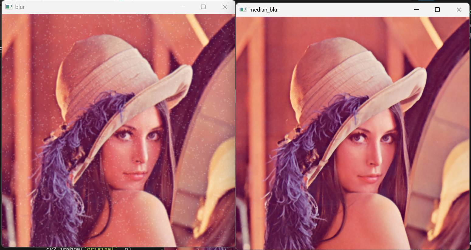
import numpy as np
import cv2
image =cv2.imread('image/lenaNoise.png')
# image = cv2.imread('./image/mybaby.jpg')

cv2.imshow('Original', image)

# stack output images together
blurred = np.hstack([cv2.medianBlur(image, 3),
                     cv2.medianBlur(image, 5),
                     cv2.medianBlur(image, 7)])

cv2.imshow('MedianBlue 3, 5, 7', cv2.resize(blurred, None, fx=0.75, fy=0.75))
cv2.waitKey(0)
cv2.destroyAllWindows()
cv2.waitKey(1)
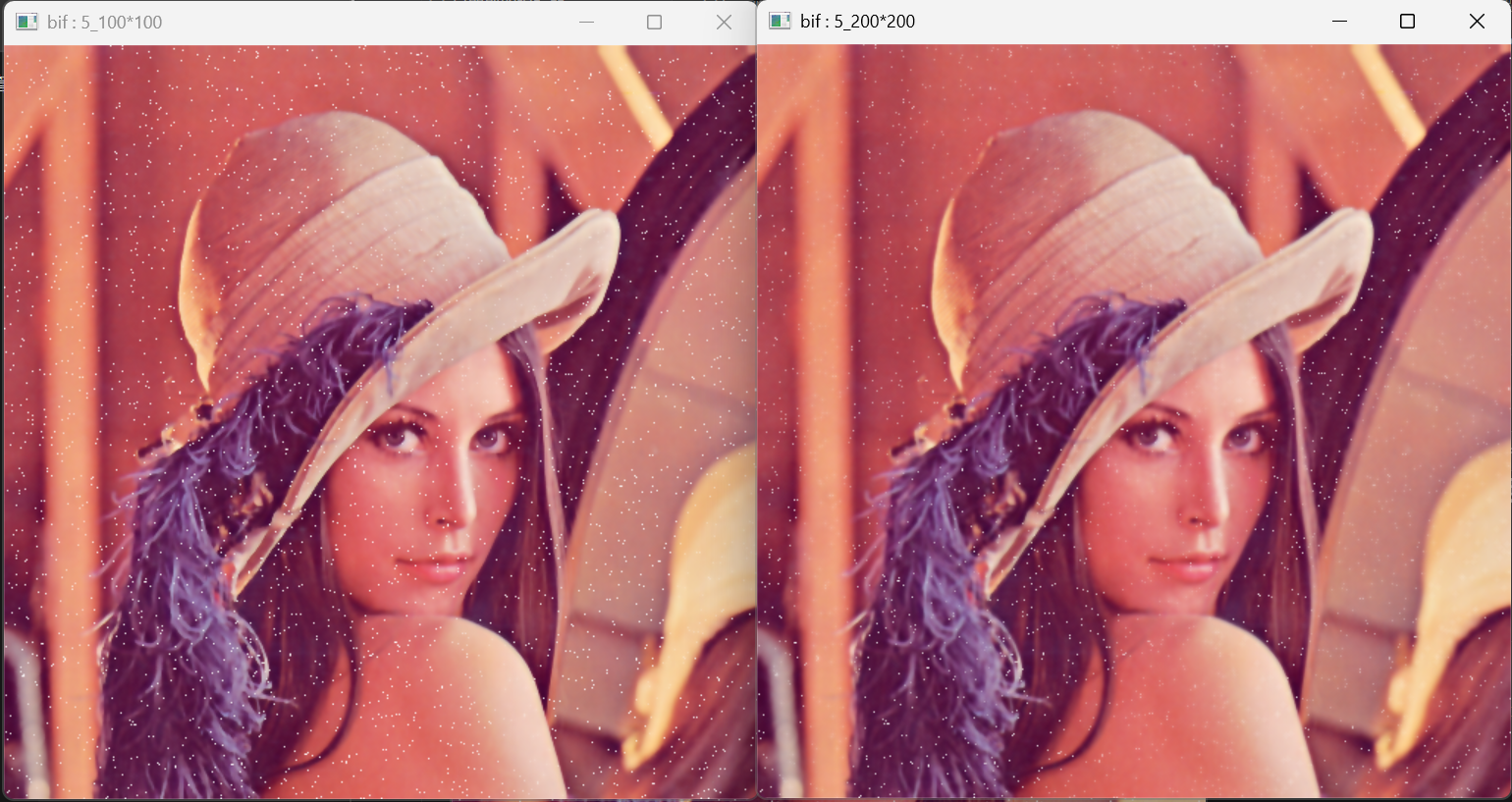
Bilateral Filter 雙邊濾波器
結合兩種權重 空間權重: 距離越近權重越大 強度權重: 與中心像素差異越大 權重越小
import cv2
o = cv2.imread('./image/lenaNoise.png')
r1 = cv2.bilateralFilter(o, 5, 100, 100)
r2 = cv2.bilateralFilter(o, 5, 200, 200)

cv2.imshow('original', o)
cv2.imshow('bif : 5_100*100', r1)
cv2.imshow('bif : 5_200*200', r2)

cv2.waitKey()
cv2.destroyAllWindows()
cv2.waitKey(1)
對雜訊的處理不如中位數濾波器
高斯濾波器 v.s. 雙邊濾波器
import cv2
o = cv2.imread('./image/bilTest.bmp')
g=r=cv2.GaussianBlur(o, (55, 55), 0, 0)
b=cv2.bilateralFilter(o, 55, 100, 100)
cv2.imshow('original',o)
cv2.imshow('Gaussian',g)
cv2.imshow('bilateral',b)
cv2.waitKey(0)
cv2.destroyAllWindows()
cv2.waitKey(1)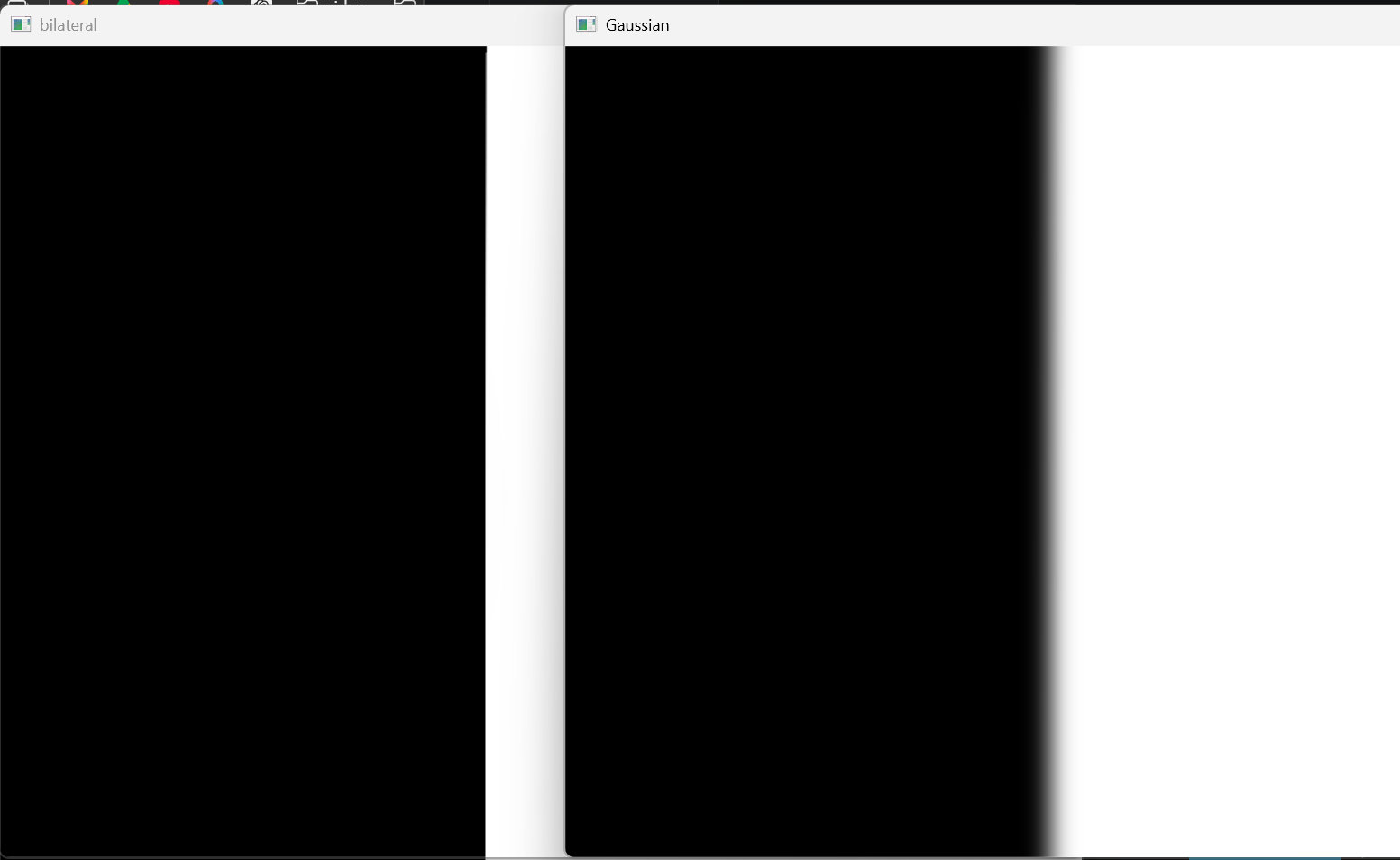 bilateralFilter 對雜訊處裡效果不好, 對邊界處理較佳
高斯濾波器考慮的是距離,距離越近,權重越大, 0 0 0 255 255 255 → 0 0 80 170 255 255 所以邊界被模糊
雙邊濾波器考慮的是距離跟顏色差異,距離越近、顏色差異越大,權重越重 0 0 0 255 255 255 → 0 0 0 255 255 255 因為顏色差異大,所以不會被平均掉 保留邊界
import numpy as np
import cv2

image = cv2.imread('./image/mybaby.jpg')
cv2.imshow('Original', image)

image=cv2.resize(image,(500, 280))

# stack output images together
blurred = np.hstack([cv2.bilateralFilter(image, 5, 20, 20),
                     cv2.bilateralFilter(image, 7, 40, 40),
                     cv2.bilateralFilter(image, 9, 60, 60)])

cv2.imshow('Bilateral', blurred)
cv2.waitKey(0)
cv2.destroyAllWindows()
cv2.waitKey(1)
影像二值化
cv2.threshold()
它會根據設定的門檻值 thresh 將像素分成兩類,並依照 type 決定如何輸出。最常用的是 THRESH_BINARY,當像素值大於門檻時設為 maxval(通常是 255),否則設為 0。這是影像分割、OCR、輪廓偵測前常見的前處理步驟。
ret, dst = cv2.threshold(
    src, # 影像
    thresh, # 門檻值
    maxval, # 超過門檻要給的值
    type # 決定如何二值化
)| Type | \> thresh | ≤ thresh | 功能 |
| THRESH_BINARY | maxval(指定值) | 0 | 標準二值化 |
| THRESH_BINARY_INV | 0 | maxval | 反向二值化 |
| THRESH_TRUNC | thresh | 原值 | 超過門檻截斷 |
| THRESH_TOZERO | 原值 | 0 | 保留亮區 |
| THRESH_TOZERO_INV | 0 | 原值 | 保留暗區 |
ret, binary = cv2.threshold( gray, 127, 255, cv2.THRESH_BINARY )
範例
```python
import cv2
import numpy as np
from matplotlib import pyplot as plt

img=np.random.randint(100, 150, size=[5, 5], dtype=np.uint8)
print(f'img : \n{img}\n')

thd, t1 = cv2.threshold(img, 125, 245, cv2.THRESH_BINARY)   # try 125
print(f'thd : {thd}\n\n'
      f't1 :\n{t1}')
img :
[[136 140 100 113 134]
[120 129 123 128 106]
[109 112 110 105 118]
[133 137 132 146 110]
[109 145 122 114 121]]
thd : 125.0
t1 :
[[245 245 0 0 245]
[ 0 245 0 245 0]
[ 0 0 0 0 0]
[245 245 245 245 0]
[ 0 245 0 0 0]]處理灰階圖
import cv2
import numpy as np

# img = cv2.resize(cv2.imread('./image/thresh.jpg', 0), (300,200))
img = cv2.resize(cv2.imread('./image/lenaColor.png', 0),(400, 300))

ret, thresh1 = cv2.threshold(img, 127, 255, cv2.THRESH_BINARY)  # 1=255, 0=0
ret, thresh2 = cv2.threshold(img, 127, 255, cv2.THRESH_BINARY_INV)
ret, thresh3 = cv2.threshold(img, 127, 255, cv2.THRESH_TRUNC)   # 1=127 Thresh, 0=value
ret, thresh4 = cv2.threshold(img, 127, 255, cv2.THRESH_TOZERO)  # 1=value,  0=0
ret, thresh5 = cv2.threshold(img, 127, 255, cv2.THRESH_TOZERO_INV)

titles = ['Original Image', 'BINARY', 'BINARY_INV', 'TRUNC', 'TOZERO', 'TOZERO_INV']
images = [img, thresh1, thresh2, thresh3, thresh4, thresh5]

plt.figure(figsize=(16, 8))

for idx, (t, i) in enumerate(zip(titles, images)):
    plt.subplot(2, 3, idx + 1)
    plt.setp(plt.title(t), color='k')
    plt.xticks([]), plt.yticks([])
    plt.imshow(i, cmap='gray', vmin=0, vmax=255)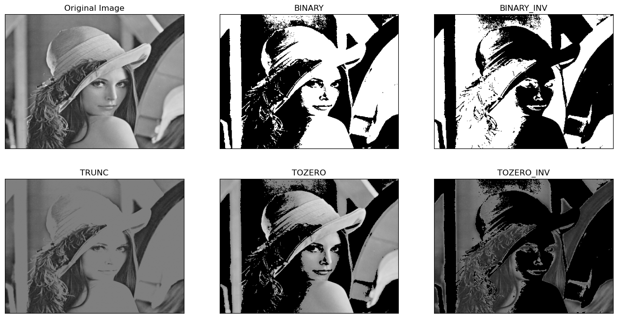
處理彩色圖
import cv2
import numpy as np

img = cv2.cvtColor(cv2.resize(cv2.imread('./image/lenaColor.png', 1),(400, 300)), cv2.COLOR_BGR2RGB)

ret, thresh1 = cv2.threshold(img, 127, 255, cv2.THRESH_BINARY)  # 1=255, 0=0
ret, thresh2 = cv2.threshold(img, 127, 255, cv2.THRESH_BINARY_INV)
ret, thresh3 = cv2.threshold(img, 127, 255, cv2.THRESH_TRUNC)   # 1=127 Thresh, 0=value
ret, thresh4 = cv2.threshold(img, 127, 255, cv2.THRESH_TOZERO)  # 1=value,  0=0
ret, thresh5 = cv2.threshold(img, 127, 255, cv2.THRESH_TOZERO_INV)

titles = ['Original Image', 'BINARY', 'BINARY_INV', 'TRUNC', 'TOZERO', 'TOZERO_INV']
images = [img, thresh1, thresh2, thresh3, thresh4, thresh5]

plt.figure(figsize=(16, 8))

for idx, (t, i) in enumerate(zip(titles, images)):
    plt.subplot(2, 3, idx + 1)
    plt.setp(plt.title(t), color='k')
    plt.xticks([]), plt.yticks([])
    plt.imshow(i)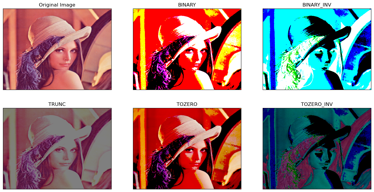
threshold adaptive ``局部`` 自我調節設定
Threshold → 大家共用一個門檻 **threshold adaptive → **每個區域自己決定門檻大小
cv2.adaptiveThreshold(
    src,  # 影像 通常是灰階圖
    maxValue, #255
    adaptiveMethod,  # 如何計算閾值
    thresholdType, # 二值化方式 通常cv2.THRESH_BINARY 或 cv2.THRESH_BINARY_INV
    blockSize, # 區域大小(奇數)
    C #門檻修正值
)
adaptiveMethod 計算方式
-
ADAPTIVE_THRESH_MEAN_C Threshold = 區域平均值 - c
-
ADAPTIVE_THRESH_GAUSSIAN_C Threshold = 高斯加權平均值 - c
blockSize : 計算局部門檻值時,我要參考多大的範圍 範圍越小,細節越多,但不容易模糊雜訊 一定要是奇數,不然會找不到中心 範例:
import cv2
import numpy as np

img=np.random.randint(0, 256, size=[6, 8], dtype=np.uint8)

print(f'img :\n{img}\n')

t1, thd = cv2.threshold(img, 127, 255, cv2.THRESH_BINARY)   # try 127 → 125
print(f'threshHold : {t1}\n\n'
      f'thd :\n{thd}\n')

# blockSize=3, C=0 (mean - C)
Ad_thd_mean = cv2.adaptiveThreshold(img, 255, cv2.ADAPTIVE_THRESH_MEAN_C, cv2.THRESH_BINARY, 3, 0)
print(f'Ad_thd_mean :\n{Ad_thd_mean}\n')

Ad_thd_gauss = cv2.adaptiveThreshold(img, 255, cv2.ADAPTIVE_THRESH_GAUSSIAN_C, cv2.THRESH_BINARY, 3, 0)
print(f'Ad_thd_gauss :\n{Ad_thd_mean}')
img :
[[ 36 206 157 205 208 154 148 174]
[ 30 11 39 19 86 132 82 99]
[115 46 144 156 122 90 66 252]
[ 90 8 15 116 223 13 73 204]
[138 142 226 159 90 217 210 166]
[ 6 57 25 101 211 194 10 57]]
threshHold : 127.0
thd :
[[ 0 255 255 255 255 255 255 255]
[ 0 0 0 0 0 255 0 0]
[ 0 0 255 255 0 0 0 255]
[ 0 0 0 0 255 0 0 255]
[255 255 255 255 0 255 255 255]
[ 0 0 0 0 255 255 0 0]]
Ad_thd_mean :
[[ 0 255 255 255 255 255 255 255]
[ 0 0 0 0 0 255 0 0]
[255 0 255 255 255 0 0 255]
[ 0 0 0 0 255 0 0 255]
[255 255 255 255 0 255 255 255]
[ 0 0 0 0 255 255 0 0]]
...
[255 0 255 255 255 0 0 255]
[ 0 0 0 0 255 0 0 255]
[255 255 255 255 0 255 255 255]
[ 0 0 0 0 255 255 0 0]]import numpy as np
import cv2
image = cv2.imread('./image/mybaby.jpg', 0)
cv2.imshow('Original', image)
ret, thresh = cv2.threshold(image, 127, 255, cv2.THRESH_BINARY) # 1 : 255, 0 : 0
cv2.imshow(f'Thresh hold {ret}, 255', thresh)
thresh = cv2.adaptiveThreshold(image, 255, cv2.ADAPTIVE_THRESH_MEAN_C, cv2.THRESH_BINARY, 5, 4)
cv2.imshow('adaptive / Mean Thresh', thresh)
thresh = cv2.adaptiveThreshold(image, 255, cv2.ADAPTIVE_THRESH_GAUSSIAN_C, cv2.THRESH_BINARY, 5, 4)
cv2.imshow('adaptive / Gaussian Thresh', thresh)
cv2.waitKey(0)
cv2.destroyAllWindows()
cv2.waitKey(1)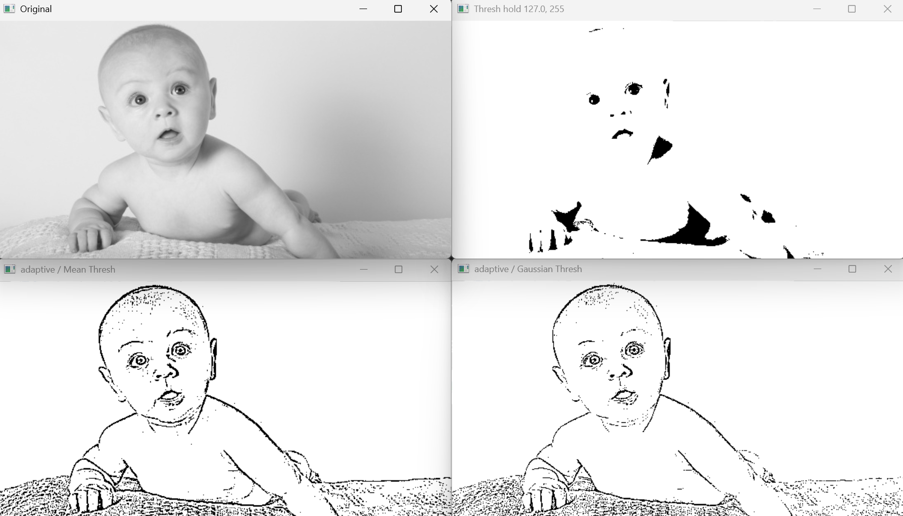
Threshold otsu (二值化自動找最佳門檻)
會根據圖片的灰階分布自動計算 Threshold。
ret, thresh = cv2.threshold(
gray,
0,
255,
cv2.THRESH_BINARY + cv2.THRESH_OTSU
)
黑色區域 白色區域
██████ ██████
██████ ██████
██████ ██████
0 120 255
otsu 會自己去找最適合把兩群資料分開的閾值
otsu的目標
讓類別內變異最小
讓類別間變異最大
範例 隨機矩陣
import cv2
import numpy as np

img=np.random.randint(0, 256, size=[6, 8], dtype=np.uint8)
print(f'img : \n{img}\n')

th2, img2 = cv2.threshold(img, 0, 255, cv2.THRESH_OTSU)  # type

#th2, img2 = cv2.threshold(img, 0, 255, cv2.THRESH_BINARY + cv2.THRESH_OTSU)
print(f'THRESH_OTSU th2 : {th2}\n\n'
      f'img2 :\n{img2}')
img :
[[ 81 165 0 114 183 53 81 34]
[165 207 19 169 109 14 22 46]
[ 58 129 232 158 70 194 49 229]
[105 19 62 84 55 153 107 92]
[ 23 24 129 119 98 116 76 88]
[107 120 6 167 166 88 125 192]]
THRESH_OTSU th2 : 98.0
img2 :
[[ 0 255 0 255 255 0 0 0]
[255 255 0 255 255 0 0 0]
[ 0 255 255 255 0 255 0 255]
[255 0 0 0 0 255 255 0]
[ 0 0 255 255 0 255 0 0]
[255 255 0 255 255 0 255 255]]範例圖
讀灰階圖
↓
固定127二值化
↓
Otsu自動找Threshold
↓
顯示兩種結果
↓
畫灰階直方圖
↓
在直方圖上標示
Otsu找到的位置
↓
把原圖放到小視窗
# using cv2 module
import numpy as np
from matplotlib import pyplot as plt
import cv2
image = cv2.imread('./image/mybaby.jpg', 0)
# image = cv2.imread('./image/lenaColor.png', 0)
cv2.imshow('original', image)
ret, thresh = cv2.threshold(image, 127, 255, cv2.THRESH_BINARY) # 1 : 255, 0 : 0
cv2.imshow('Thresh hold : 127', thresh)
# Otsu threshold
th2, img2 = cv2.threshold(image, 0, 255, cv2.THRESH_OTSU)
print(f"Otsu's threshold : {th2}")
cv2.imshow(f'Otsu : {th2}', img2)
fig=plt.figure(figsize=(10, 4))
ax0 = fig.add_axes([0.1, 0.1, 0.8, 0.8]) # 建立小視窗 # main axes
ax0.hist(image.flatten(), 256) # 畫直方圖
ax0.axvline(x=th2, color='r', lw=1)
# print(plt.ylim()[1])
ax0.text(th2+5, plt.ylim()[1]*.9, f'Otsu : {th2}', fontsize=10, color='r')
ax1 = fig.add_axes([0.12, 0.6, 0.25, 0.25]) # inside axes
ax1.imshow(cv2.cvtColor(image, cv2.COLOR_BGR2RGB))
ax1.axis('off')
cv2.waitKey(0)
cv2.destroyAllWindows()
cv2.waitKey(1)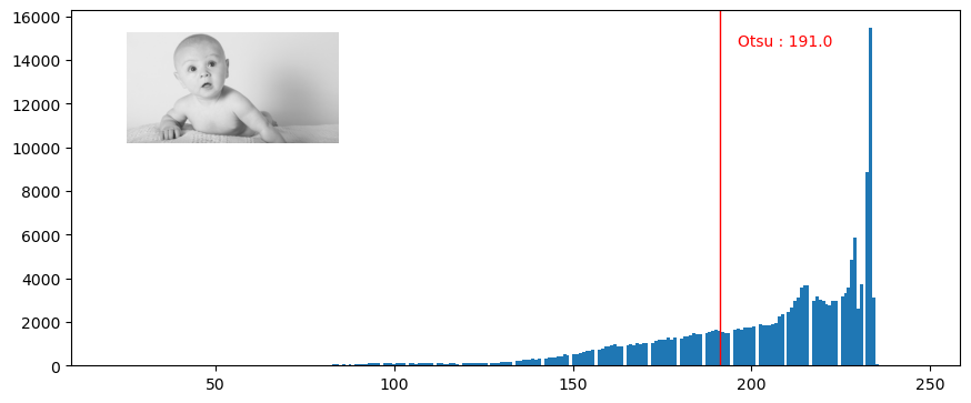 Otsu’s threshold : 191.0
Edge detection 邊緣偵測
openCV 提供三種邊緣檢測方式來處理 `Sobel、Canny 及 Laplacian`,這些技術皆是使用 `灰階` 的影像,基於每個像素灰度的不同,利用不同物體在其邊界處會`有明顯的邊緣特徵來分辨`。這三種方法皆使用了`一維甚至於二維的微分`,嚴格來說,若依其使用技術原理的不同可分為兩種:
1. Sobel 和 Canny 使用的則是 Gradient methods(梯度原理),它是透過計算像素光度的`一階導數差異`(detect changes in the first derivative of intensity)來進行邊緣檢測。
10 10 10 10 200 200 → 做一階微分 → 0 0 0 190 0
Sobel X:
[[-1,0,1],
 [-2,0,2],
 [-1,0,1]]
10 10 200
10 10 200
10 10 200
(-1×10)+(0×10)+(1×200)
+
(-2×10)+(0×10)+(2×200)
+
(-1×10)+(0×10)+(1×200)
= 760
得到一個很大的值,表示亮度變化很劇烈
Sobel 的梯度
Gx: 水平方向
[[-1,0,1],
[-2,0,2],
[-1,0,1]]
Gy: 垂直方向
[[-1,-2,-1],
 [ 0, 0, 0],
 [ 1, 2, 1]]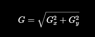
- Laplacian 原稱為 Laplacian method,透過計算零交越點上光度的`二階導數`(detect zero crossings of the second derivative on intensity changes)
| 函數 | 功能 |
| `np.abs()` | 只取絕對值 |
| `cv2.convertScaleAbs()` | 取絕對值 + 轉 uint8 + 限制 0\~255 |
Sobel 濾波器
會先找sobelX,再找sobleY,最後再用cv2.addWeighted()合併
cv2.Sobel(
    src, # 影像
    ddepth, # 影像深度
    dx,  # x方向導數階數
    dy,  # y方向導數階數
    ksize=3, # kernel size
    scale=1, # 縮放倍率
    delta=0, # 額外加值
    borderType=cv2.BORDER_DEFAULT #邊界處理方式
)| dx | dy | 意義 |
| 1 | 0 | Gx (X方向梯度) |
| 0 | 1 | Gy (Y方向梯度) |
| 1 | 1 | 同時計算X與Y二階混合導數(較少用) |
ddept = -1 unit8 的單邊解釋
img = np.zeros((7, 7), dtype=np.uint8)
img[1:6, 1:6] = 10  # padding problem = 10
print(f'img :\n{img}\n')

sobelx = cv2.Sobel(img, -1, 1, 0, ksize=-1)  # ddepth = -1, dx=1, dy=0
sobely = cv2.Sobel(img, -1, 0, 1, ksize=-1)  # ddepth = -1, dx=0, dy=1
sobelxy = cv2.addWeighted(sobelx, 0.5, sobely, 0.5, 0)  # dst = src1*alpha + src2*beta + gamma;

print(f'sobelx uint8 :\n{sobelx}\n\n'
      f'sobely uint8 :\n{sobely}\n\n'
      f'sobelxy :\n{sobelxy}\n')
img :
[[ 0 0 0 0 0 0 0]
[ 0 10 10 10 10 10 0]
[ 0 10 10 10 10 10 0]
[ 0 10 10 10 10 10 0]
[ 0 10 10 10 10 10 0]
[ 0 10 10 10 10 10 0]
[ 0 0 0 0 0 0 0]]
sobelx uint8 :
[[ 0 60 0 0 0 0 0]
[ 0 130 0 0 0 0 0]
[ 0 160 0 0 0 0 0]
[ 0 160 0 0 0 0 0]
[ 0 160 0 0 0 0 0]
[ 0 130 0 0 0 0 0]
[ 0 60 0 0 0 0 0]]
sobely uint8 :
[[ 0 0 0 0 0 0 0]
[ 60 130 160 160 160 130 60]
[ 0 0 0 0 0 0 0]
[ 0 0 0 0 0 0 0]
[ 0 0 0 0 0 0 0]
[ 0 0 0 0 0 0 0]
...
[ 0 80 0 0 0 0 0]
[ 0 65 0 0 0 0 0]
[ 0 30 0 0 0 0 0]]ksize = -1 → Scharr Kernel X方向:
 -3   0   3
-10   0  10
 -3   0   3
Y方向:
 -3 -10 -3
  0   0  0
  3  10  3
Scharr 是專門優化 3×3 Sobel 的梯度估計,因此在 3×3 Kernel 下通常比 Sobel 更精準。但 Scharr 只能使用固定的 3×3 Kernel,而 Sobel 可以使用 3×3、5×5、7×7 等不同大小的 Kernel。當影像雜訊較多時,較大的 Sobel Kernel 能提供更好的平滑效果,因此兩者各有適用場景。
ddepth = cv2.CV_64F 雙邊解譯
img = np.zeros((7, 7), dtype=np.uint8)
img[1:6, 1:6] = 10
print(f'img :\n{img}\n')

sobelx = cv2.Sobel(img, cv2.CV_64F, 1, 0)   # ddepth = cv2.CV64F
sobely = cv2.Sobel(img, cv2.CV_64F, 0, 1)   # ddepth = cv2.CV64F

sobelx = cv2.convertScaleAbs(sobelx)        # 絕對值, 轉換為cv2.CV_8U
sobely = cv2.convertScaleAbs(sobely)        # 絕對值, 轉換為cv2.CV_8U
sobelxy = cv2.addWeighted(sobelx, 0.5, sobely, 0.5, 0)

print(f'sobelx CV_64F :\n{sobelx}\n\n'
      f'sobely CV_64F :\n{sobely}\n\n'
      f'sobelxy :\n{sobelxy}\n')
img :
[[ 0 0 0 0 0 0 0]
[ 0 10 10 10 10 10 0]
[ 0 10 10 10 10 10 0]
[ 0 10 10 10 10 10 0]
[ 0 10 10 10 10 10 0]
[ 0 10 10 10 10 10 0]
[ 0 0 0 0 0 0 0]]
sobelx CV_64F :
[[ 0 20 0 0 0 20 0]
[ 0 30 0 0 0 30 0]
[ 0 40 0 0 0 40 0]
[ 0 40 0 0 0 40 0]
[ 0 40 0 0 0 40 0]
[ 0 30 0 0 0 30 0]
[ 0 20 0 0 0 20 0]]
sobely CV_64F :
[[ 0 0 0 0 0 0 0]
[20 30 40 40 40 30 20]
[ 0 0 0 0 0 0 0]
[ 0 0 0 0 0 0 0]
[ 0 0 0 0 0 0 0]
[20 30 40 40 40 30 20]
...
[ 0 20 0 0 0 20 0]
[10 30 20 20 20 30 10]
[ 0 10 0 0 0 10 0]]unit8 v.s. CV_64F
因為 unit8 的範圍只有0~255 ,不存負值,所以soble出來的值,如果有負數就會變成0,邊緣就會少掉一邊
CV_64F 可以存負值,所以負值邊緣會被保留下來
最重要的事的,做完要做convertScaleAbs(),取絕對值轉回unit8,才有辦法以影像形式顯示。
Sobel 使用 CV_64F 是為了保留梯度計算中的負值與避免溢位,但 Sobel 的輸出代表梯度而不是影像亮度,因此無法直接作為一般影像顯示。最後通常會使用 cv2.convertScaleAbs() 將梯度取絕對值並轉換成 uint8 (0~255),讓邊緣強度能夠以影像形式顯示或儲存。
| 型態 | 範圍 |
| uint8 | 0 \~ 255 |
| int16 | -32768 \~ 32767 |
| float32 | ±3.4 × 10³⁸ |
| float64 | ±1.8 × 10³⁰⁸ |
sobelx = cv2.Sobel(o, cv2.CV_16S, 1, 0) # ddepth = cv2.CV_16S, dx=1, dy=0,
sobelx = cv2.Sobel(o, cv2.CV_64F, 1, 0) # ddepth = cv2.CV64V
sobelx = cv2.convertScaleAbs(sobelx) # 絕對值, 轉換為cv2.CV_8U
sobely = cv2.Sobel(o, cv2.CV_64F, 0, 1) # ddepth = cv2.CV_64V, dx=0, dy=1, sobely = cv2.convertScaleAbs(sobely) # 絕對值, 轉換為 cv2.CV_8U
sobelxy_or = cv2.bitwise_or(sobelx, sobely)
sobelxy_and = cv2.bitwise_and(sobelx, sobely)
cv2.imshow(‘original’, o) cv2.imshow(‘x CV_16S’, sobelx) cv2.imshow(‘y CV_16S’, sobely) cv2.imshow(‘xy_or’, sobelxy_or)
cv2.imshow(‘xy_and’, sobelxy_and)
cv2.waitKey() cv2.destroyAllWindows() cv2.waitKey(1)
## **Scharr 濾波器**
charr 濾波器是對 Sobel 運算元差異性的增強,兩者之間的在檢測圖像邊緣的原理和使用方式上相同。而 Scharr 濾波器的主要思路是通過將模版中的`權重係數放大來增大圖元值間的差異`。
```python
cv2.Scharr(
    src, # 影像
    ddepth, # 輸出型態
    dx, # x的導數階數
    dy,  # y的導數階數
    scale=1, # 縮放倍率
    delta=0, # 偏移植
    borderType=cv2.BORDER_DEFAULT #邊界填補方式
)
import cv2
import numpy as np
# o = cv2.imread('./image/sobel.bmp')
o = cv2.imread('./image/lenaColor.png') # 微分更敏感
scharrx = cv2.Scharr(o, cv2.CV_64F, 1, 0) # try dx=1, dy=1
scharry = cv2.Scharr(o, cv2.CV_64F, 0, 1)
# scharrx = cv2.Scharr(o, cv2.CV_16S, 1, 0) # try dx=1, dy=1
# scharry = cv2.Scharr(o, cv2.CV_16S, 0, 1)
# scharrx = cv2.Scharr(o, -1, 1, 0) # try dx=1, dy=1
# scharry = cv2.Scharr(o, -1, 0, 1)
scharrx = cv2.convertScaleAbs(scharrx) # 轉回uint8
scharry = cv2.convertScaleAbs(scharry) # 轉回uint8
scharrxy = cv2.addWeighted(scharrx, 0.5, scharry, 0.5, 0)
cv2.imshow('original',o)
cv2.imshow('scharr x', scharrx)
cv2.imshow('scharr y', scharry)
cv2.imshow('xy',scharrxy)
cv2.waitKey()
cv2.destroyAllWindows()
cv2.waitKey(1)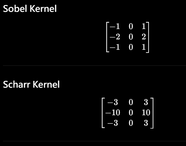 Sobel:
中間權重 = 2
Scharr:
中間權重 = 10
Scharr 梯度權重更高,定位越精準
cv2.Scharr(img, cv2.CV_64F, 1, 0)

cv2.Sobel(img, cv2.CV_64F, 1, 0, ksize=-1)

ksize=-1 會直接用Scharr來計算
所以上述兩種是等價的寫法
** Sobel vs. Scharr**
import cv2
o = cv2.imread('./image/lenaColor.png')
# =========== Sobel ======================
sobelx = cv2.Sobel(o, cv2.CV_64F, 1, 0, ksize=3)
sobely = cv2.Sobel(o, cv2.CV_64F, 0, 1, ksize=3)
sobelx = cv2.convertScaleAbs(sobelx)
sobely = cv2.convertScaleAbs(sobely)
sobelxy = cv2.addWeighted(sobelx, 0.5, sobely, 0.5, 0)
# ========== Scharr ======================
scharrx = cv2.Scharr(o, cv2.CV_64F,1,0)
scharry = cv2.Scharr(o, cv2.CV_64F,0,1)
scharrx = cv2.convertScaleAbs(scharrx)
scharry = cv2.convertScaleAbs(scharry)
scharrxy = cv2.addWeighted(scharrx, 0.5,scharry, 0.5, 0)
cv2.imshow('original', o)
cv2.imshow('sobel_xy', sobelxy)
cv2.imshow('scharr_xy', scharrxy)
cv2.waitKey()
cv2.destroyAllWindows()
cv2.waitKey(1)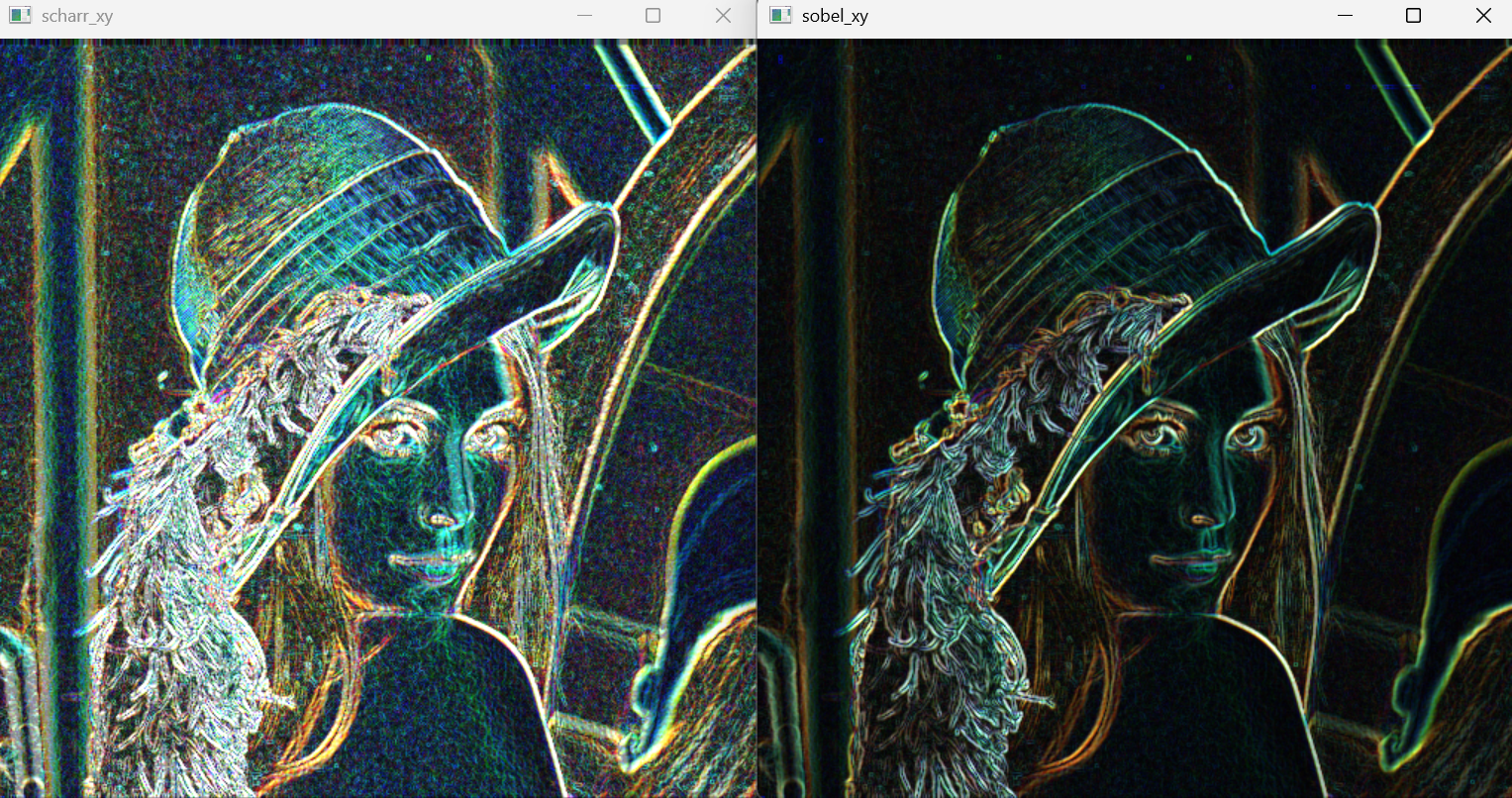 Scharr 可以視為 Sobel 在 3×3 Kernel 下的改良版本。它使用經過最佳化的權重,因此對影像梯度的估計更準確,邊界定位通常比 Sobel(3×3) 更好。不過 Scharr 只能使用固定的 3×3 Kernel,而 Sobel 可以使用 5×5、7×7 等較大的 Kernel,在高雜訊環境下反而可能有更好的穩定性。
Laplacian
用二階導數找邊緣
Laplacian對於雜訊(Noise)非常敏感,因此在實用上都會將影像先模糊化後再處理 (LoG Laplacian of Gaussian)。
使用 Laplacian 找出邊緣。注意使用此函數除了傳入灰階影像之外,亦須指定輸出的影像浮點格式 CV_64F
一階導數的找法
0 0 0 255 255 255 → 0 0 255 0 0 最大的位置表示邊緣
二階導數 對一階導數微分 → 雜訊會被放大 0 0 255 0 0→ 0 255 -255 0 0 Zero Crossing 零交越點: 就是正負值的交界處 255 → -255的位置
cv2.Laplacian(
    src, # 影像
    ddepth, # 影像輸出型態  通常CV_64F 因為有負值
    ksize=1, # kernel大小  預設 = 1
    scale=1, # 縮放倍率
    delta=0, # 偏移量
    borderType=cv2.BORDER_DEFAULT #邊界填補
)| 特性 | Sobel | Laplacian |
| 導數 | 一階 | 二階 |
| 邊緣定位 | 好 | 更敏感 |
| 抗雜訊 | 較佳 | 較差 |
| 方向性 | 有(X/Y) | 全方向 |
| 計算量 | 小 | 小 |
array([[ 0, 0, 0, 0, 0, 0, 30, 0, 10, 0, 0, 0], [ 0, 0, 0, 0, 0, 20, 20, 10, 10, 0, 0, 0], [ 0, 0, 0, 0, 20, 20, 0, 10, 10, 0, 0, 0], [ 0, 0, 0, 20, 20, 0, 0, 10, 10, 0, 0, 0], [ 0, 0, 20, 20, 0, 0, 0, 10, 10, 0, 0, 0], [ 0, 10, 30, 0, 0, 0, 0, 10, 10, 0, 0, 0]], dtype=uint8)
圖例
```python
import cv2
# o = cv2.imread('./image/sobel.bmp')
o = cv2.imread('./image/lenaColor.png',1)
o=cv2.blur(o, (3,3))
# cv2.imshow('blur', o)

Laplacian = cv2.Laplacian(o, cv2.CV_64F, ksize=3)   # ksize=1 default
Laplacian = cv2.convertScaleAbs(Laplacian)

cv2.imshow('original', o)
cv2.imshow('Laplacian', Laplacian)

cv2.waitKey()
cv2.destroyAllWindows()
cv2.waitKey(1)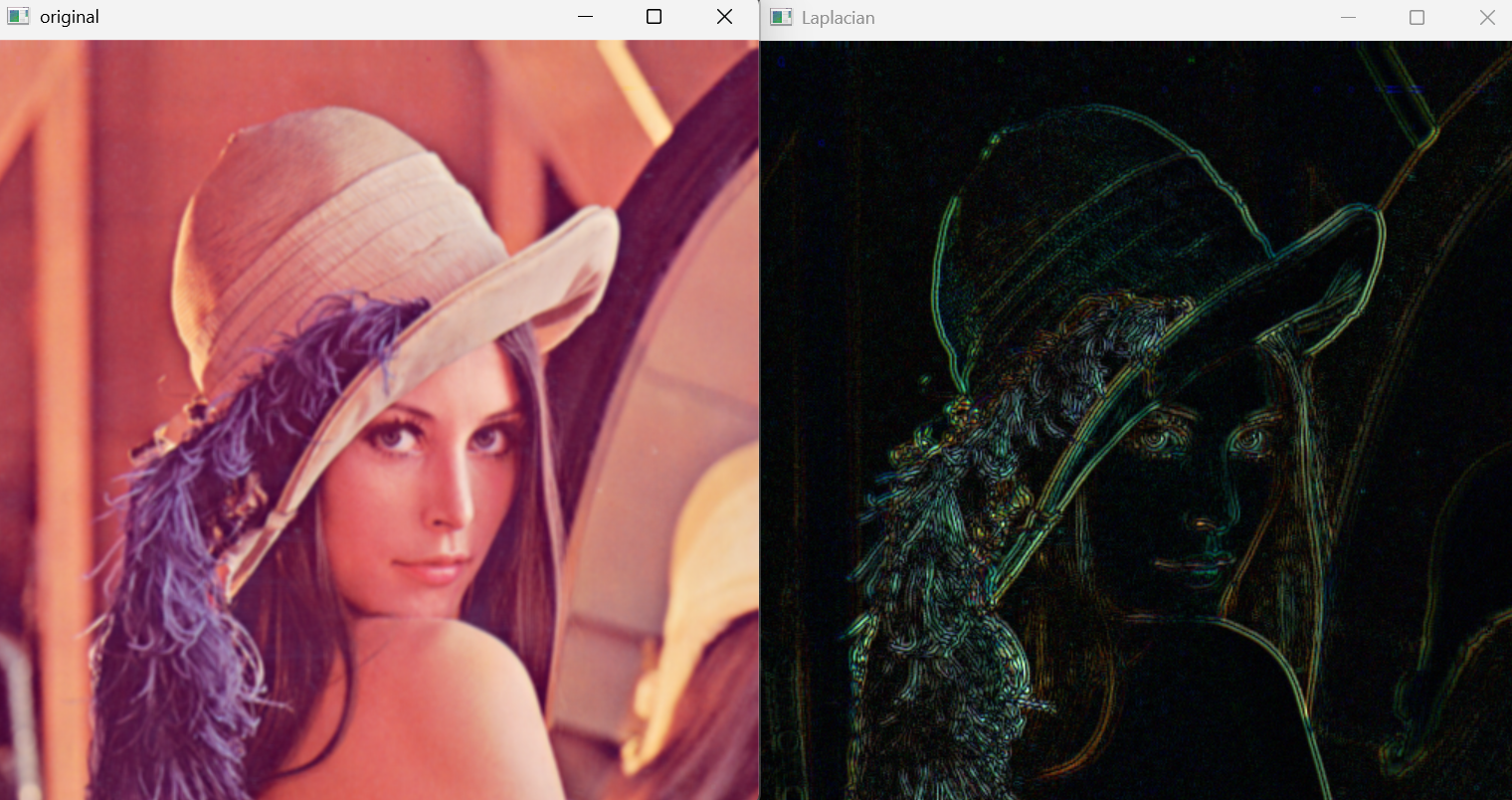
| 特性 | Sobel | Laplacian |
| 邊界清晰度 | ★★★★★ | ★★★ |
| 邊界方向 | 有 | 無 |
| 雜訊敏感度 | 中 | 高 |
| 邊界定位 | 好 | 很細 |
| 常用程度 | 很高 | 較少單獨使用 |
Canny 多步驟邊緣偵測演算法
Canny 邊緣檢測,其實 Canny 不能被單獨稱為一種方法,因為它是一連串的過程加上其它方法,先模糊化去除不必要的像素、再使用類似 Sobel 方式取得XY軸邊緣。它先將影像模糊化再進行非極大值抑制(non-maxima suppression),因此 Canny 比起 Sobel 較能處理雜訊問題,但是需要花費較多的硬體資源來處理。在下方的實作中我們可以看到它們輸出的差異。
語法
edge = cv2.Canny(
    image,
    threshold1, # 低門檻
    threshold2, # 高門檻
    apertureSize=3,  # Sobel Kernel大小
L2gradient=True # 算剃度的方式 T-> 用開根號, F->用絕對值
)
必做步驟
- Gaussian Blur → 去除雜訊
blur = cv2.GaussianBlur(
    img,
    (5,5),
    0
)- Sobel 梯度
- Non-Maximum Suppression (NMS) → 將變界的線條變細 需要知道邊緣的方向
- Double Threshold 兩個閾值 ex: 100 200 >200 就是強邊界,保留 100 < 閾值 <200 就是若邊界,先標記 <100 刪除
- Edge Tracking
檢查弱邊界有沒有連接到強邊界,有則保留,否則刪除,達到去除孤立雜訊的效果。
Canny =
Gaussian Blur
↓
Sobel(Gx,Gy)
↓
Magnitude + Direction
↓
NMS(邊界細化)
↓
Double Threshold
↓
Hysteresis Tracking
↓
Edge Image
| 特性 | Sobel | Canny |
| 去雜訊 | ❌ | ✔ |
| 邊界細化 | ❌ | ✔ |
| 雙門檻 | ❌ | ✔ |
| 邊界連通 | ❌ | ✔ |
| 邊界品質 | 普通 | 很好 |
範例:
import numpy as np
import cv2
img = np.zeros((8, 8), dtype=np.uint8)
img[1:7, 1:7] = 10  # padding problem = 10
print(f'img :\n{img}\n')

sobelx = cv2.Sobel(img, cv2.CV_32F, 1, 0, ksize=-1)  # ddepth = -1, dx=1, dy=0
sobely = cv2.Sobel(img, cv2.CV_32F, 0, 1, ksize=-1)  # ddepth = -1, dx=0, dy=1
# 找邊緣的強度、方向
mag, angle = cv2.cartToPolar(sobelx, sobely, angleInDegrees=True)
sobelxy = cv2.addWeighted(sobelx, 0.5, sobely, 0.5, 0)

print(f'sobelx :\n{sobelx}\n\n'
      f'sobely :\n{sobely}\n\n'
      f'mag :\n{mag.round(0)}\n\n'
      f'angle 0, 45, 90, 135.... :\n{angle.round(0)}\n\n'
      f'sobelxy :\n{sobelxy}\n')

img :
[[ 0  0  0  0  0  0  0  0]
 [ 0 10 10 10 10 10 10  0]
 [ 0 10 10 10 10 10 10  0]
 [ 0 10 10 10 10 10 10  0]
 [ 0 10 10 10 10 10 10  0]
 [ 0 10 10 10 10 10 10  0]
 [ 0 10 10 10 10 10 10  0]
 [ 0  0  0  0  0  0  0  0]]

sobelx :
[[   0.   60.    0.    0.    0.    0.  -60.    0.]
 [   0.  130.    0.    0.    0.    0. -130.    0.]
 [   0.  160.    0.    0.    0.    0. -160.    0.]
 [   0.  160.    0.    0.    0.    0. -160.    0.]
 [   0.  160.    0.    0.    0.    0. -160.    0.]
 [   0.  160.    0.    0.    0.    0. -160.    0.]
 [   0.  130.    0.    0.    0.    0. -130.    0.]
 [   0.   60.    0.    0.    0.    0.  -60.    0.]]

sobely :
[[   0.    0.    0.    0.    0.    0.    0.    0.]
 [  60.  130.  160.  160.  160.  160.  130.   60.]
 [   0.    0.    0.    0.    0.    0.    0.    0.]
 [   0.    0.    0.    0.    0.    0.    0.    0.]
...
 [   0.   80.    0.    0.    0.    0.  -80.    0.]
 [ -30.    0.  -80.  -80.  -80.  -80. -130.  -30.]
 [   0.   30.    0.    0.    0.    0.  -30.    0.]]

 mag :
[[  0.  60.   0.   0.   0.   0.  60.   0.]
 [ 60. 184. 160. 160. 160. 160. 184.  60.]
 [  0. 160.   0.   0.   0.   0. 160.   0.]
 [  0. 160.   0.   0.   0.   0. 160.   0.]
 [  0. 160.   0.   0.   0.   0. 160.   0.]
 [  0. 160.   0.   0.   0.   0. 160.   0.]
 [ 60. 184. 160. 160. 160. 160. 184.  60.]
 [  0.  60.   0.   0.   0.   0.  60.   0.]]

 sobelxy :
[[   0.   30.    0.    0.    0.    0.  -30.    0.]
 [  30.  130.   80.   80.   80.   80.    0.   30.]
 [   0.   80.    0.    0.    0.    0.  -80.    0.]
 [   0.   80.    0.    0.    0.    0.  -80.    0.]
 [   0.   80.    0.    0.    0.    0.  -80.    0.]
 [   0.   80.    0.    0.    0.    0.  -80.    0.]
 [ -30.    0.  -80.  -80.  -80.  -80. -130.  -30.]
[ 0. 30. 0. 0. 0. 0. -30. 0.]]| 梯度角度 | 分類方向 |
| 0° \~ 22.5° | 0° |
| 22.5° \~ 67.5° | 45° |
| 67.5° \~ 112.5° | 90° |
| 112.5° \~ 157.5° | 135° |
↓
得到 Gx、Gy cartToPolar
↓
得到 mag、angle angle.round(0)
↓
方便觀察梯度方向 Canny NMS
↓
通常會把角度量化成
0°、45°、90°、135°
img=np.array([
[30 ,30 ,30 ,30 ,30 ,30 ,30 ,20 ,10 ,10 ,10 ,10],
[30 ,30 ,30 ,30 ,30 ,30 ,20 ,20 ,10 ,10 ,10 ,10],
[30 ,30 ,30 ,30 ,30 ,20 ,20 ,20 ,10 ,10 ,10 ,10],
[30 ,30 ,30 ,30 ,20 ,20 ,20 ,20 ,10 ,10 ,10 ,10],
[30 ,30 ,30 ,20 ,20 ,20 ,20 ,20 ,10 ,10 ,10 ,10],
[30 ,30 ,20 ,20 ,20 ,20 ,20 ,20 ,10 ,10 ,10 ,10]], dtype='uint8')
canny = cv2.Canny(img, 15, 30)
# Laplacian = cv2.Laplacian(img, cv2.CV_16S)  # error
# Laplacian = cv2.convertScaleAbs(Laplacian)
canny

array([[  0,   0,   0,   0,   0,   0,   0, 255,   0,   0,   0,   0],
       [  0,   0,   0,   0,   0, 255, 255,   0,   0,   0,   0,   0],
       [  0,   0,   0,   0, 255, 255,   0, 255,   0,   0,   0,   0],
       [  0,   0,   0, 255, 255,   0,   0, 255,   0,   0,   0,   0],
       [  0,   0, 255, 255,   0,   0,   0, 255,   0,   0,   0,   0],
       [  0,   0, 255,   0,   0,   0,   0, 255,   0,   0,   0,   0]],
      dtype=uint8)
cv2.cartToPolar() 用來將 Sobel 計算出的 X、Y 梯度 (Gx, Gy) 轉換成極座標形式。其中 mag 表示梯度大小,計算公式為 sqrt(Gx² + Gy²);angle 表示梯度方向,計算公式為 atan2(Gy, Gx)。在 Canny 邊緣偵測中,mag 用來判斷邊緣強度,而 angle 則用於 Non-Maximum Suppression 判斷邊緣方向。
Canny vs. Sobel
import cv2
o = cv2.imread('./image/lenaColor.png', 0)
# o = cv2.imread('./image/contour.png', 1)
# o = cv2.imread('./image/coins.jpg',0)

r1=cv2.Canny(o, 50, 150)   # different threshold
r2=cv2.Canny(o, 32, 96)    # different threshold

sobelx = cv2.Sobel(o, cv2.CV_64F, 1, 0, ksize=3)
sobely = cv2.Sobel(o, cv2.CV_64F, 0, 1, ksize=3)

sobelx = cv2.convertScaleAbs(sobelx)   # 轉回 Uint8
sobely = cv2.convertScaleAbs(sobely)
sobelxy = cv2.addWeighted(sobelx, 0.5, sobely, 0.5, 0)

cv2.imshow('original', o)
cv2.imshow('Canny r50_150', r1)
cv2.imshow('Canny r32_96', r2)
cv2.imshow('sobel_xy', sobelxy)

cv2.waitKey()
cv2.destroyAllWindows()
cv2.waitKey(1)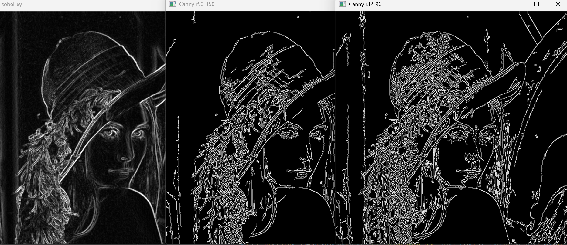
Canny : road edge detect
import numpy as np
import cv2

image = cv2.imread('./image/road1.jpg', 1)
image = cv2.resize(image, (750, 450), interpolation=cv2.INTER_AREA)
# image = cv2.GaussianBlur(image, (5, 5), 0)  # 弱化雜訊
cv2.imshow('Blurred', image)

# Canny edge detection
canny = cv2.Canny(image, 30, 150, apertureSize=3, L2gradient=0) # threshold1=39, threshhold2=150, sobel size=3
cv2.imshow('Canny', canny)

cv2.waitKey(0)
cv2.destroyAllWindows()
cv2.waitKey(1)
Video with canny
### import numpy as np
import cv2

cap = cv2.VideoCapture(0)

## Define the codec and create VideoWriter object
fourcc = cv2.VideoWriter_fourcc(*'XVID')
# out = cv2.VideoWriter('./video/output.avi',fourcc, 20.0, (640,480))  # 20 FPS, size=640, 480

while(cap.isOpened()):
    ret, frame = cap.read()
    frame = cv2.Canny(frame, 100, 200)
    if ret==True:
        frame = cv2.flip(frame,1)

# write the flipped frame
#         out.write(frame)
        cv2.imshow('frame', frame)

        if cv2.waitKey(1) == 27:
            break
    else:
        break

## Release everything if job is finished
cap.release()
# out.release()
cv2.destroyAllWindows()
cv2.waitKey(1)
Sobel vs. Laplacian vs. Canny
import numpy as np
import cv2

# image = cv2.imread('./image/coins.jpg', 1)
image = cv2.imread('./image/road1.jpg', 0)       # road edge detection

cv2.imshow('Original', image)

# ===== Sobel edge detection ============
sobelX = cv2.Sobel(image, cv2.CV_64F, 1, 0)
sobelY = cv2.Sobel(image, cv2.CV_64F, 0, 1)

sobelX = cv2.convertScaleAbs(sobelX)
sobelY = cv2.convertScaleAbs(sobelY)
sobelXY = cv2.addWeighted(sobelX, 0.5, sobelY, 0.5, 0)
th2, sobelXY = cv2.threshold(sobelXY, 0, 255,  cv2.THRESH_OTSU)

# ===== Laplacian edge detection ========
lap = cv2.Laplacian(image, cv2.CV_64F)
lap = cv2.convertScaleAbs(lap)
th2, lap = cv2.threshold(lap, 0, 255,  cv2.THRESH_OTSU)

# ===== Canny edge detection ============
canny=cv2.Canny(image, 32, 128)    # different threshold

cv2.imshow('Sobel X', sobelX)
cv2.imshow('Sobel Y', sobelY)
cv2.imshow('Sobel XY after threshold', sobelXY)
cv2.imshow('Laplacian after threshold', lap)
cv2.imshow('canny', canny)

cv2.waitKey(0)
cv2.destroyAllWindows()
cv2.waitKey(1)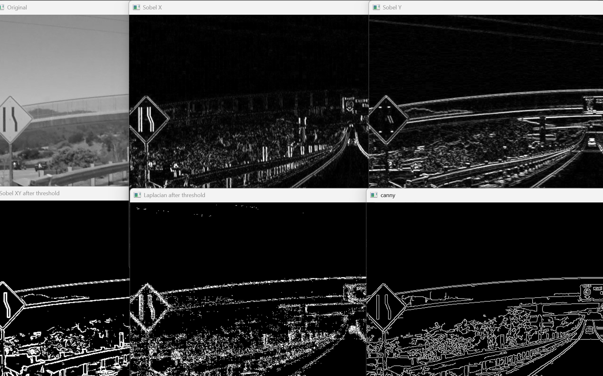
DoG (Difference of Gaussian)
Gaussian Blur : 看低頻 DoG: 兩個不同模糊程度相減,留下高頻資訊,因此會強調邊緣與細節
import numpy as np
import cv2

# img = cv2.imread('./image/lenaColor.png',0)
img = cv2.imread('./image/opencv.jpg',1)
d=5
img_D03 = cv2.GaussianBlur(img, (d, d), 0.3)
img_D05 = cv2.GaussianBlur(img, (d, d), 0.5)
img_D07 = cv2.GaussianBlur(img, (d, d), 0.7)
img_D09 = cv2.GaussianBlur(img, (d, d), 0.9)
img_D11 = cv2.GaussianBlur(img, (d, d), 1.1)
img_D13 = cv2.GaussianBlur(img, (d, d), 1.3)

img_D05_03 = img_D05 - img_D03
img_D09_07 = img_D09 - img_D07
img_D11_13 = img_D11 - img_D13

cv2.imshow('img', img)
cv2.imshow('DoG05_03', img_D05_03)
cv2.imshow('DoG09_07', img_D09_07)
cv2.imshow('DoG11_13', img_D11_13)
cv2.waitKey(0)
cv2.destroyAllWindows()
cv2.waitKey(1)
import numpy as np
import cv2
# img = cv2.imread('./image/lenaColor.png')
img = cv2.imread('./image/opencv.jpg',1)
img_G0 = cv2.GaussianBlur(img, (3, 3),1) # 𝜎𝑥 = 𝜎𝑦 = 0.8
img_G1 = cv2.GaussianBlur(img, (5, 5),1) # 𝜎𝑥 = 𝜎𝑦 = 1.1
img_DoG = img_G0 - img_G1 # try img_G0 + img_G1
cv2.imshow('img', img)
cv2.imshow('DoG', img_DoG)
cv2.waitKey(0)
cv2.destroyAllWindows()
cv2.waitKey(1)img → imgG0 → img_G1 with same filter
import numpy as np
import cv2

# img = cv2.imread('./image/lenaColor.png')
img = cv2.imread('./image/opencv.jpg',1)

img_G0 = cv2.GaussianBlur(img, (3, 3),1)      # img  => img_G0
img_G1 = cv2.GaussianBlur(img_G0, (3, 3),1)

img_DoG = img_G0 - img_G1   # try img_G0 + img_G1

cv2.imshow('img', img)
cv2.imshow('DoG', img_DoG)
cv2.waitKey(0)
cv2.destroyAllWindows()
cv2.waitKey(1)
輪廓偵測 (contours)
流程:
灰階
↓
Threshold
↓
findContours
因為 findContours 需要明確的前景與背景,因此通常會先將灰階影像進行二值化處理。
cv2.findContours
contours, hierarchy = cv2.findContours(
    image,
    mode, #輪廓檢索模式
    method  #輪廓點儲存方式
)
Mode
| Mode | 語法 | 功能 | 是否保留階層 |
| 外部輪廓 | `cv2.RETR_EXTERNAL` | 只找最外層輪廓 | ❌ |
| 全部輪廓 | `cv2.RETR_LIST` | 找所有輪廓 | ❌ |
| 兩層結構 | `cv2.RETR_CCOMP` | 分成外輪廓與內輪廓兩層 | ⭕ |
| 樹狀結構 | `cv2.RETR_TREE` | 找所有輪廓並建立完整父子關係 | ⭕ |
| FloodFill | `cv2.RETR_FLOODFILL` | 配合 FloodFill 使用,較少用 | ⭕ |
| Method | 語法 | 說明 | 記憶體 |
| 保留全部點 | `cv2.CHAIN_APPROX_NONE` | 所有輪廓點全部保存 | 大 |
| 簡化輪廓 | `cv2.CHAIN_APPROX_SIMPLE` | 只保留轉折點 | 小 |
| Teh-Chin L1 | `cv2.CHAIN_APPROX_TC89_L1` | 輪廓近似演算法 | 更小 |
| Teh-Chin KCOS | `cv2.CHAIN_APPROX_TC89_KCOS` | 改良版輪廓近似 | 更小 |
contourIdx
| 值 | 意義 |
| -1 | 畫全部輪廓 |
| 0 | 畫第0個輪廓 |
| 1 | 畫第1個輪廓 |
| n | 畫第n個輪廓 |
img_1 = cv2.drawContours(im.copy(), cnts, -1, (0, 255, 0), 2) # image, contour, contouridx, (color), thickness img0 = cv2.drawContours(im.copy(), cnts, 0, (0, 255, 0), 2) # image, contour, contouridx, (color), thickness img1 = cv2.drawContours(im.copy(), cnts, 1, (0, 255, 0), 2) # image, contour, contouridx, (color), thickness img2 = cv2.drawContours(im.copy(), cnts, 2, (0, 255, 0), 2) # image, contour, contouridx, (color), thickness img3 = cv2.drawContours(im.copy(), cnts, 3, (0, 255, 0), 2) # image, contour, contouridx, (color), thickness
print (f’contours 型別\t\t: {type(cnts)}\n’ f’第 0 個contours\t\t: {type(cnts[0])}\n’ f’contours 數量\t\t: {len(cnts)}\n’)
for i in range(len(cnts)): print (f’contours[{i}]儲存點的個數\t: {len(cnts[i])}’)
cv2.imshow(‘imgray’, imgray) cv2.imshow(‘thresh’, thresh) cv2.imshow(‘img_1’, img_1) cv2.imshow(‘img0’, img0) cv2.imshow(‘img1’, img1) cv2.imshow(‘img2’, img2) cv2.imshow(‘img3’, img3) # 第三個不見了
cv2.waitKey(0) cv2.destroyAllWindows() cv2.waitKey(1)
配合二值化檢測
```python
import numpy as np
import cv2
imgray = cv2.imread('./image/contour.png', 0)

ret, thresh = cv2.threshold(imgray, 225, 255, cv2.THRESH_BINARY_INV)  # try cv2.THRESH_BINARY

cnts, hierarchy = cv2.findContours(thresh, cv2.RETR_EXTERNAL, cv2.CHAIN_APPROX_SIMPLE)
print(f'Next, Previous, First_Child, Parent\n {hierarchy}\n')        # [next, previous, First_Child, Parent]

cntsImg=[]
for i in range(len(cnts)):
    # temp=np.zeros(imgray.shape, np.uint8)
    temp=np.zeros_like(imgray, np.uint8) #建立同尺寸的黑布
    cntsImg.append(temp)
    cntsImg[i]=cv2.drawContours(cntsImg[i], cnts, i, (255,255,255), 3)
    cv2.imshow('contours['+ str(i)+']', cntsImg[i])

cv2.imshow('imgray', imgray)
cv2.imshow('thresh', thresh)

cv2.waitKey()
cv2.destroyAllWindows()
cv2.waitKey(1)
cv2.RETR_TREE : 建立一個等級樹結構的輪廓
import numpy as np
import cv2
im = cv2.imread('./image/contour.png')
imgray = cv2.cvtColor(im, cv2.COLOR_BGR2GRAY)
ret, thresh = cv2.threshold(imgray, 127, 255, cv2.THRESH_BINARY_INV)

cnts, hierarchy = cv2.findContours(thresh, cv2.RETR_TREE, cv2.CHAIN_APPROX_SIMPLE)
# cnts, hierarchy = cv2.findContours(thresh, cv2.RETR_LIST, cv2.CHAIN_APPROX_NONE)
print(f'Next, Previous, First_Child, Parent\n {hierarchy}\n')        # [next, previous, First_Child, Parent]

for i in range(-1, len(cnts)) :
    img = cv2.drawContours(im.copy(), cnts, i, (0, 255, 0), 2) # image, contour, contouridx, (color), thickness
    cv2.imshow(f'img{i}', img)
    if i >=0 : print (f'contours[{i}]儲存點的個數\t: {len(cnts[i])}')

print (f'\ncontours 型別\t\t: {type(cnts)}\n'
       f'第 0 個contours\t\t: {type(cnts[0])}\n'
       f'contours 數量\t\t: {len(cnts)}\n')

cv2.imshow('imgray', imgray)
cv2.imshow('thresh', thresh)

cv2.waitKey(0)
cv2.destroyAllWindows()
cv2.waitKey(1)
boundingRect
import cv2

src = cv2.imread("./image/contour.png")
cv2.imshow("src", src)
src_gray = cv2.cvtColor(src,cv2.COLOR_BGR2GRAY)     # 影像轉成灰階

ret, dst_binary = cv2.threshold(src_gray, 127, 255, cv2.THRESH_BINARY_INV)  # 二值化處理影像
# 找尋影像內的輪廓
contours, hierarchy = cv2.findContours(dst_binary, cv2.RETR_LIST, cv2.CHAIN_APPROX_SIMPLE)
lt = 16
for i in range(len(contours)):
    x, y, w, h = cv2.boundingRect(contours[i])        # 建構矩形  會回傳四個值
    print(f'contour[{i}]左上角\t\tx = {x}\n'
          f'contour[{i}]左上角\t\ty = {y}\n'
          f'contour[{i}]矩形寬度\tw = {w}\n'
          f'contour[{i}]矩形高度\th = {h}\n')

    dst = cv2.rectangle(src,(x, y),(x+w, y+h),(0,0,255),2)
    cv2.putText(dst, f'w/h : {w/h:.2f}', (x, y-5), 2, .6, (0,0,255), 1, lt)
cv2.imshow("dst",dst)

cv2.waitKey(0)
cv2.destroyAllWindows()
cv2.waitKey(1)
畫矩形
cv2.rectangle(
    image,
    pt1, #左上角座標
    pt2, #右下角座標
    color,
    thickness
)
矩形上寫字
cv2.putText(
    image,
    text,
    org,  # 文字起始座標 文字左下角的那個點
    font, # 字型
    fontScale, # 字型大小
    color,  # 顏色
    thickness, # 線寬
    lineType # 抗鋸齒 預設:cv2.LINE_AA
)
openCV 字型
| 常數 | 說明 |
| `cv2.FONT_HERSHEY_SIMPLEX` | 最常用 |
| `cv2.FONT_HERSHEY_PLAIN` | 細字 |
| `cv2.FONT_HERSHEY_DUPLEX` | 雙線字 |
| `cv2.FONT_HERSHEY_COMPLEX` | 較正式 |
| `cv2.FONT_HERSHEY_TRIPLEX` | 粗體風格 |
| `cv2.FONT_HERSHEY_SCRIPT_SIMPLEX` | 手寫風格 |
矩的計算
影像識別的一個核心問題是影像的特徵提取,簡單描述即為用一組簡單的資料(資料描述量)來描述整個影像,這組資料愈簡單越有代表性越好。良好的特徵不受光線、噪點、幾何形變的干擾,影像識別技術的發展中,不斷有新的描述影像特徵提出,而影像不變 矩 就是其中一個。
從影像中計算出來的 矩 通常描述了影像不同種類的幾何特徵如:大小、灰度、方向、形狀等,影像矩廣泛應用於模式識別、目標分類、目標識別與防偽估計、影像編碼與重構等領域。
讀取圖片 ↓ 二值化 ↓ 找輪廓 ↓ 畫出輪廓 ↓ 計算每個輪廓的 Moments ↓ 利用 m00 求面積
import numpy as np
import cv2

im = cv2.imread("./image/contour.png")
cv2.imshow('original', im)

imgray = cv2.cvtColor(im, cv2.COLOR_BGR2GRAY)
ret, thresh = cv2.threshold(imgray, 225, 255, cv2.THRESH_BINARY)  # try cv2.THRESH_BINARY

cnts, hierarchy = cv2.findContours(thresh, cv2.RETR_LIST, cv2.CHAIN_APPROX_SIMPLE)
print(f'next, previous, First_Child, Parent\n {hierarchy}\n')        # [next, previous, First_Child, Parent]

cntsImg=cv2.drawContours(im.copy(), cnts, -1, (0,255,0), 3)
cv2.imshow('contours', cntsImg)

print('觀察各輪廓的矩(moments) :\n')
for i in range(len(cnts)):
    print(f'輪廓 {i} 的矩 :\n{cv2.moments(cnts[i])}\n')

print('觀察各輪廓的面積 :\n')
for i in range(len(cnts)):
    print(f"輪廓 {i} 的面積\t: {cv2.moments(cnts[i])['m00']:>10,.1f}")

cv2.waitKey()
cv2.destroyAllWindows()
cv2.waitKey(1)